Fall 2016, CS-116A Lecture: Splines

Splines
CS-116A: Introduction to Computer Graphics
Instructor: Rob Bruce
Fall 2016

SLIDE 1: Bézier curve

Invented by French engineer, Pierre Bézier (1910-1999).
Advantages: Draw a smooth curve through a series of linear interpolations.

SLIDE 2: Bézier curve: Application

Where could Bézier curves be used?
To draw smooth, vector-based typefaces like Microsoft TrueType or Adobe Postscript.
In computer aided design (CAD).
In paint and draw programs.

SLIDE 3: n degree Bézier curve

Bézier curves with n = 1 are called degree 1 polynomials (linear) and have two control points: P₀ (x,y) and P₁ (x,y).
Bézier curves with n = 2 are called degree 2 polynomials (quadratic) and have three control points: P₀ (x,y), P₁ (x,y), and P₂ (x,y).
Bézier curves with n = 3 are called degree 3 polynomials (cubic) and have four control points: P₀ (x,y), P₁ (x,y), P₂ (x,y), and P₃ (x,y).
Bézier curves with n = 4 are called degree 4 polynomials (quartic) and have five control points: P₀ (x,y), P₁ (x,y), P₂ (x,y), P₃ (x,y), and P₄ (x,y).
etc.

The general formula for Bézier curves of degree n is:
$\sum_{i = 0}^{n} (\begin{matrix} n \\ i \end{matrix}) * {(1 - t)}^{n - i} * t^{i} * w_{i}$

w_i are constants (weights). These weights are either the X or Y value for each control point, P_n (x,y)
$(\begin{matrix} n \\ i \end{matrix})$ represents the binomial coefficients (i.e. a given row of Pascal's triangle). For example, the binomial coefficients for n = 3 are: 1, 3, 3, 1
A cubic Bézier curve (n = 3) can be written as the parametric equation:
1 * (1 - t)³ * w₀ + 3 * (1 - t)² * t * w₁ + 3 * (1 - t) * t² * w₂ + 1 * t³ * w₃
You will be using 3rd degree (cubic) Bézier curves in your paint/draw program.

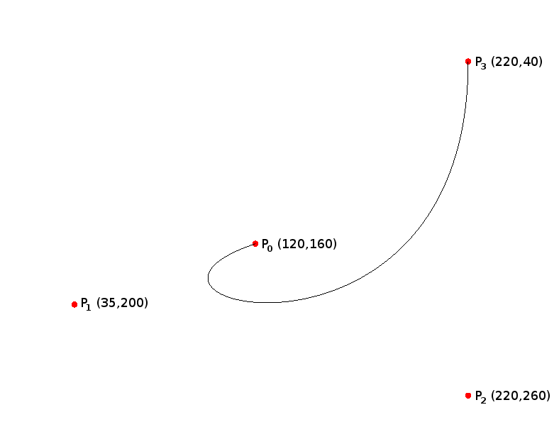
SLIDE 4: Example Bézier curve (n = 3)

A third degree Bézier curves contains the following four control points: P₀: (120, 160); P₁: (35, 200); P₂: (220, 260); P₃: (220, 40)
To plot the (x,y) points for this Bézier curve in OpenGL, we can compute the cubic Bézier curve's X and Y components for a given value of t.
X = (1 - t)^(3-0) * t⁰ * 1 * 120 + (1 - t)^(3-1) * t¹ * 3 * 35 + (1 - t)^(3-2) * t² * 3 * 220 + (1 - t)^(3-3) * t³ * 1 * 220
Y = (1 - t)^(3-0) * t⁰ * 1 * 160 + (1 - t)^(3-1) * t¹ * 3 * 200 + (1 - t)^(3-2) * t² * 3 * 260 + (1 - t)^(3-3) * t³ * 1 * 40

SLIDE 5: Dissecting our example Bézier curve (n = 3)

Notice the binomial coefficients (1, 3, 3, 1) for the cubic Bézier curve:
X = (1 - t)^(3-0) * t⁰ * 1 * 120 + (1 - t)^(3-1) * t¹ * 3 * 35 + (1 - t)^(3-2) * t² * 3 * 220 + (1 - t)^(3-3) * t³ * 1 * 220
Y = (1 - t)^(3-0) * t⁰ * 1 * 160 + (1 - t)^(3-1) * t¹ * 3 * 200 + (1 - t)^(3-2) * t² * 3 * 260 + (1 - t)^(3-3) * t³ * 1 * 40

SLIDE 6: Dissecting our example Bézier curve (n = 3)

Notice the numbers in bold come from the X values of the four control points P₀: (120, 160); P₁: (35, 200); P₂: (220, 260); P₃: (220, 40) defining our cubic Bézier curve:
X = (1 - t)^(3-0) * t⁰ * 1 * 120 + (1 - t)^(3-1) * t¹ * 3 * 35 + (1 - t)^(3-2) * t² * 3 * 220 + (1 - t)^(3-3) * t³ * 1 * 220

SLIDE 7: Dissecting our example Bézier curve (n = 3)

Notice the numbers in bold come from the Y values of the four control points P₀: (120, 160); P₁: (35, 200); P₂: (220, 260); P₃: (220, 40) defining our cubic Bézier curve:
Y = (1 - t)^(3-0) * t⁰ * 1 * 160 + (1 - t)^(3-1) * t¹ * 3 * 200 + (1 - t)^(3-2) * t² * 3 * 260 + (1 - t)^(3-3) * t³ * 1 * 40

SLIDE 8: Example Bézier curve (n = 3): solving for t

To compute the X and Y values for our Bézier curve, we must iterate over values of t from 0 to 1 inclusive:
X = (1 - t)^(3-0) * t⁰ * 1 * 120 + (1 - t)^(3-1) * t¹ * 3 * 35 + (1 - t)^(3-2) * t² * 3 * 220 + (1 - t)^(3-3) * t³ * 1 * 220
Y = (1 - t)^(3-0) * t⁰ * 1 * 160 + (1 - t)^(3-1) * t¹ * 3 * 200 + (1 - t)^(3-2) * t² * 3 * 260 + (1 - t)^(3-3) * t³ * 1 * 40
t = 0: x = 120; y = 160
t = 0.25: x = ?; y = ?
t = 0.5: x = ?; y = ?
t = 1: x = 220; y = 40
Notice the computed X and Y values for t = 0 and t = 1 match those of P₀ and P₃. For a cubic Bézier curve, these control points are always on our curve while the middle two control points (P₁ and P₂) are never on the curve.

SLIDE 9: Plot of example Bézier curve (n = 3) with control points

Image of a Bezier curve with labled control points at (120,160), (35,200); (220,260), and (220,40).

SLIDE 10: Continuity

Two Bézier curves can be joined together.
Smoothness of curve at juncture point determined by continuity: C⁰, C¹, and C².
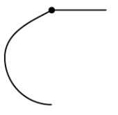
C⁰ continuity:
Curves are joined together and share a common point.
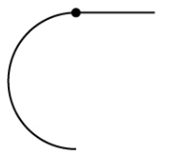
C¹ continuity:
First derivative at juncture point of both curves is equal.
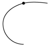
C² continuity:
First and second derivative at juncture point of both curves is equal.

SLIDE 11: C⁰ continuity

Image of two curves joined with C0 continuity.

SLIDE 12: C¹ continuity

Image of two curves joined with C1 continuity.

SLIDE 13: C² continuity

Image of two curves joined with C2 continuity.

SLIDE 14: Bézier curve application: typography

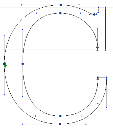
Image of a letter 'C' comprised of joined Bezier curves (typography).

Image source: http://blogs.unimelb.edu.au/sciencecommunication/files/2013/08/Twinspng_4721.png

SLIDE 15: Meshes

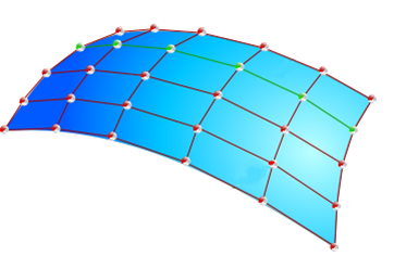
Image of a computer graphics mesh comprised of splines.

Image source: https://upload.wikimedia.org/wikipedia/commons/8/88/Surface_modelling.svg

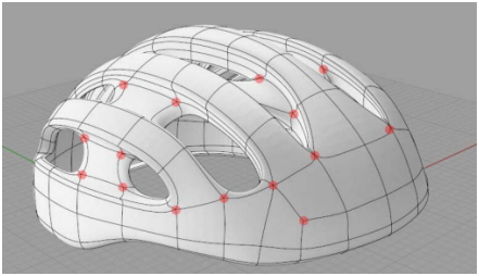
SLIDE 16: Meshes

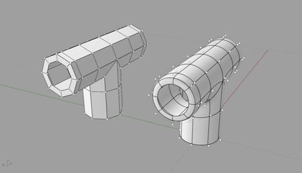
Image of T-pipes modeled from splines.

Image source: http://www.tsplines.com/UserManual_files/image059.jpg

SLIDE 17: Meshes

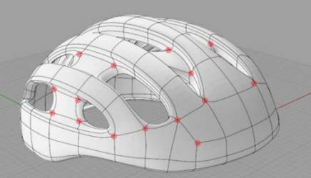
Image of a bicycle helmet modeled with splines in a mesh.

Image source: http://isicad.ru/uploads/img/2618_T-spline.PNG

SLIDE 18: Meshes

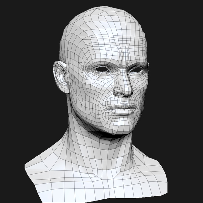
3D model of a human head comprised of splines in a mesh.

Image source: https://www.creativecrash.com/system/portfolio/photos/000/023/705/23705/big/3d_model_human_head_male_mesh.jpg?1450167195

SLIDE 19: Lathe functionality

A method for rapidly creating complex 3D objects.
Start with a 2D curve.
Spin the curve around an axis (X, Y, or Z).
Instant volume-based 3-dimensional object!

SLIDE 20: Lathe function

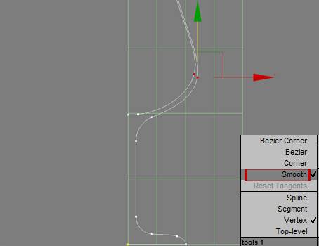
Partial contour of a wine glass modeled with splines.

Image source: http://www.3dworld-wide.com/tutorial_glass/3ds_max_spline_modeling_glass_side.jpg

SLIDE 21: Lathe function

Wine glasses modeled with splines.

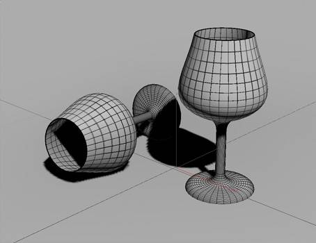
Image source: http://www.3dworld-wide.com/tutorial_glass/3ds_max_spline_modeling_glass.jpg

SLIDE 22: For further reading...

An introduction to splines for use in computer graphics and geometric modeling by Richard H. Bartels, John C. Beatty, and Brian A. Barsky
Curves and surfaces for computer aided geometric design: A practical guide by Gerald Farin
Curves and Surfaces for Computer Graphics by David Salomon
A practical guide to splines by Carl de Boor
The NURBS Book by Les A. Piegl