Chris Pollett > Students > Hammoudeh
Print View
[Home]
[Blog]
Zayd Hammoudeh's Thesis Blog:
- CS299 Week #17: October 4, 2016 Meeting
- CS299 Week #16: September 27, 2016 Meeting
- CS299 Week #15: September 20, 2016 Meeting
- CS299 Week #14: September 13, 2016 Meeting
- CS299 Week #13: September 6, 2016 Meeting
- CS297 Week #12: April 26, 2016 Meeting
- CS297 Week #11: April 19, 2016 Meeting
- CS297 Week #10: April 12, 2016 Meeting
- CS297 Week #9: April 5, 2016 Meeting
- CS297 Week #8: No Meeting due to SJSU Spring Break
- CS297 Week #7: March 22, 2016 Meeting
- CS297 Week #6: March 15, 2016 Meeting
- CS297 Week #5: March 8, 2016 Meeting
- CS297 Week #4: March 1, 2016 Meeting
- CS297 Week #3: February 23, 2016 Meeting
- CS297 Week #2: February 16, 2016 Meeting
- CS297 Week #1: February 9, 2016 Meeting
Summary of the Meeting on October 4, 2016:
This week's blog update is relatively short as I spent most of my time working on the tasks and ran out of time to work on the blog. Below is the proposed schedule for the remainder of CS299.Task Description |
Planned |
Status |
|---|---|---|
| Complete Solver and Show Full Results | Tuesday October 4 | On track |
| Submit First Thesis Draft to Dr. Pollett | Thursday October 13 | On Track |
| Experimental Result Data Collection Complete | Monday October 17 | May adjust plan |
| Complete Thesis Draft to Dr. Pollett | Tuesday October 18 | On Track |
| Distribute Thesis Draft to Committee | Monday October 24 | On Track |
| Defense | Monday October 31 | On Track |
| Submit Thesis to GAPE | Thursday November 3 | On Track |
Summary of the Meeting on September 27, 2016:
The work for this week was divided among the following activities:- Modifying the base Paikin and Tal solver to support the following:
- Solving only a subset of the pieces
- Running the solver multiple times
- Stopping the placer from running after a certain number of pieces have been placed
- Finding key segments in the original puzzle(s)
- Building a solver for the stitching pieces of each segment
- Develop a technique for determining the similarity between solved segments.
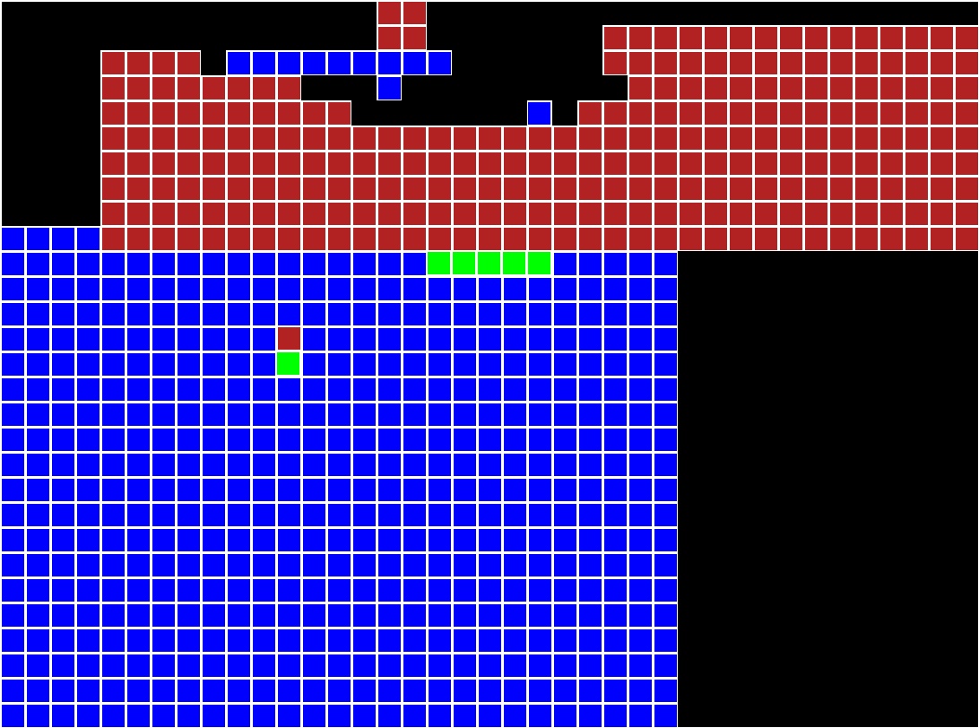
Initial Segmenter
Below is pseudocode for the implementation of the initial segmenter.saved_segments = {} unplaced_pieces = {all_pieces} do: // Run the solver and generate a single output puzzle solved_puzzle = run_single_puzzle_paikin_tal_solver(unplaced_pieces) // Segment the puzzle solved_segments = solved_puzzle.segment() max_segment_size = solved_segments.get_max_segment_size() // Save all segments at least half as large as the largest segment for each segment in solved_segments: if |segment| > max_segment_size / 2: saved_segments.append(segment) unplaced_pieces.remove_placed_pieces(segment) while max_segment_size < minimum_segment_size and |unplaced_pieces| > 0 return saved_segments
Example Solver Results
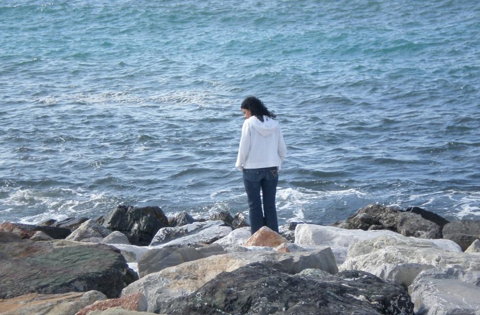
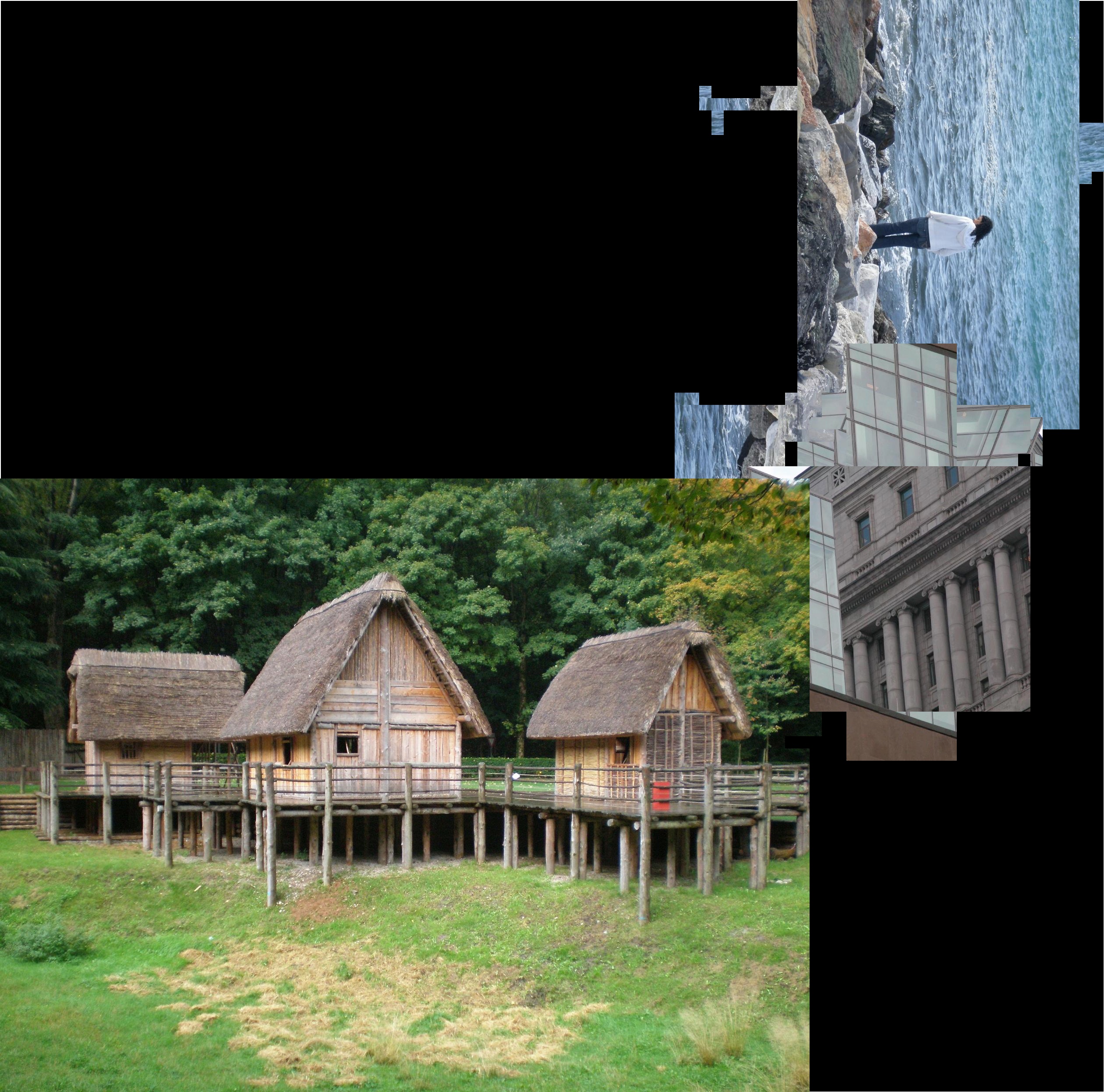
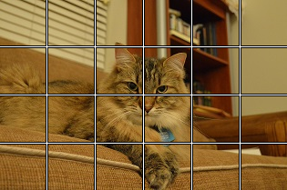
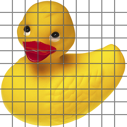
Below are three input puzzles passed to the solver.Input |
 |
 |
 |
|---|
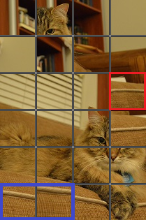
The initial segmentation solver ran four rounds. Below are the output image from each of the rounds. Note that between each round, the image is segmented and the largest segments removed. The pieces in those segments are then excluded from future placement.
Round #1 |
 |
|---|---|
Round #2 |
 |
Round #3 |
 |
Round #4 |
 |
These puzzles were then segmented into four segments with each placement round yielding a single segment. Note that while in this case each round yielded a single segment, that will not always be the case.
Segment #0 |
 |
|---|---|
Segment #1 |
 |
Segment #2 |
 |
Segment #3 |
 |
After the segments have been found, stitching pieces near the edge of each segment are indentified. This is done using the stitching piece identification algorithm described in last week's blog.
Stitching Piece Solvers
After the initial segmenter has completed, individual segments are run on each of the stitching pieces.for each segment in solved_segments: for each stitching_piece in segment.find_stitching_pieces(): output_puzzle = run_fixed_size_paikin_tal_solver(seed_piece = stitching_piece) overlap_coefficient = output_puzzle.calculate_segment_over(solved_segments) save_best_segment_scores(segment, overlap_coefficient) return best_segment_scores
Asymmetric Segment Overlap Metric
As mentioned above, a single puzzle solver of fixed size is run for each of the stitching pieces. Below is a proposed metric for quantitifying the similarity between two segments.`Overlap(\Phi_i,\Phi_j)=argmax_{\zeta_k in \Phi_i}{|P_{\zeta_k}\cap\Phi_j|}/{min(|P_{\zeta_k}|, |\Phi_j|)}`
- `\Phi_i` - `i`th segment from the initial segmentation
- `\zeta_k` - `k`th stitching piece in segment `\Phi_i`
- `P_{\zeta_k}` - Fixed size solved puzzle with stitching piece as `\zeta_k` seed.
Segment Similarity
The similarity between two segments is proposed to be:`Similarity(\Phi_i,\Phi_j)={Overlap(\Phi_i,\Phi_j)+Overlap(\Phi_j,\Phi_i)}/{2}`
Summary of the Meeting on September 20, 2016:
The work for this week was divided among the following activities:- Designing a robust algorithm for determining the distance each piece in a segment is from the nearest open space.
- Designing an algorithm to select the pieces to be used when stitching multiple segments together.
- Initial development of a modified solver that can use the segments to build
Algorithm for Determining Each Piece's Distance from an Open Space:
The goal of this algorithm is to determine for each piece the nearest open space. This can be trivially solved in O(n2) time (where n is the number of pieces in the segment). My goals in designing the algorithm where the following:- O(n) runtime (or as close to it as possible)
- Account for any spurs that may exist
- Handle any chaining because of a narrowing in the shape of the segment.
- Handle any voids in the middle of the segment (e.g., a donut effect)
- Create a visualization showing the distance of each piece from the nearest open space to check the results of the algorithm
explored_pieces = { }

locations_at_previous_distance = { all open spaces adjacent to piece }

distance_from_open = 1
while |frontier_pieces| > 0:

    locations_at_current_distance = { }

    // Use locations at distance one less to find locations at current distance
    for each prev_dist_location in locations_at_previous_distance:

        for each adjacent_loc in prev_dist_location.adjacent_location():

            // If piece is not yet explored, then minimum distance is the current one
            if has_puzzle_piece_at(adjacent_loc) && piece_id(adjacent_loc) not in explored_pieces:
                explored_pieces.delete( piece_id(adjacent_loc) )
                set_piece_distance(piece_id(adjacent_loc), distance_from_open)
                locations_at_current_distance.append(adjacent_loc)

    // Use current generation for next generation
    locations_at_previous_distance = locations_at_current_distance

    // Increment the distance from open
    distance_from_open = distance_from_open + 1
Algorithm for Determining the Piece Locations for Stitching Multiple Segments Together:
Given a set of disjoint segments, we must determine the similarity between each segment. This can be achieved by identifying a set of pieces along the edge of each segment and see if the two segments grow into one another. The algorithm here finds the set of pieces. If a stitching piece is too close to the edge of the segment, it may form specious bounds with other segments as it is known that the most likely location to have a false best buddy is along the edge of the image. What is more, if stitching piece is too far from an edge, it may never grow into a neighboring segment. It is for this reason that the algorithm finds the distance between each piece and the nearest open puzzle location. The requirements for this algorithm are similar to those for the distance algorithm. Pseudocode is below:Divide the segment into a set of square grid of disjoint cells stitching_pieces = {} for each grid_cell in { grid cells with puzzle piece adjacent to open }: cell_center = center(grid_cell) cells_at_dist = { pieces in grid_cell closest to ideal_distance_from_open } select cell_stitching_piece as piece in cells_at_dist nearest to cell_center stitching_pieces.append(nearest_piece_to_center) return stitching_pieces
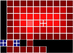
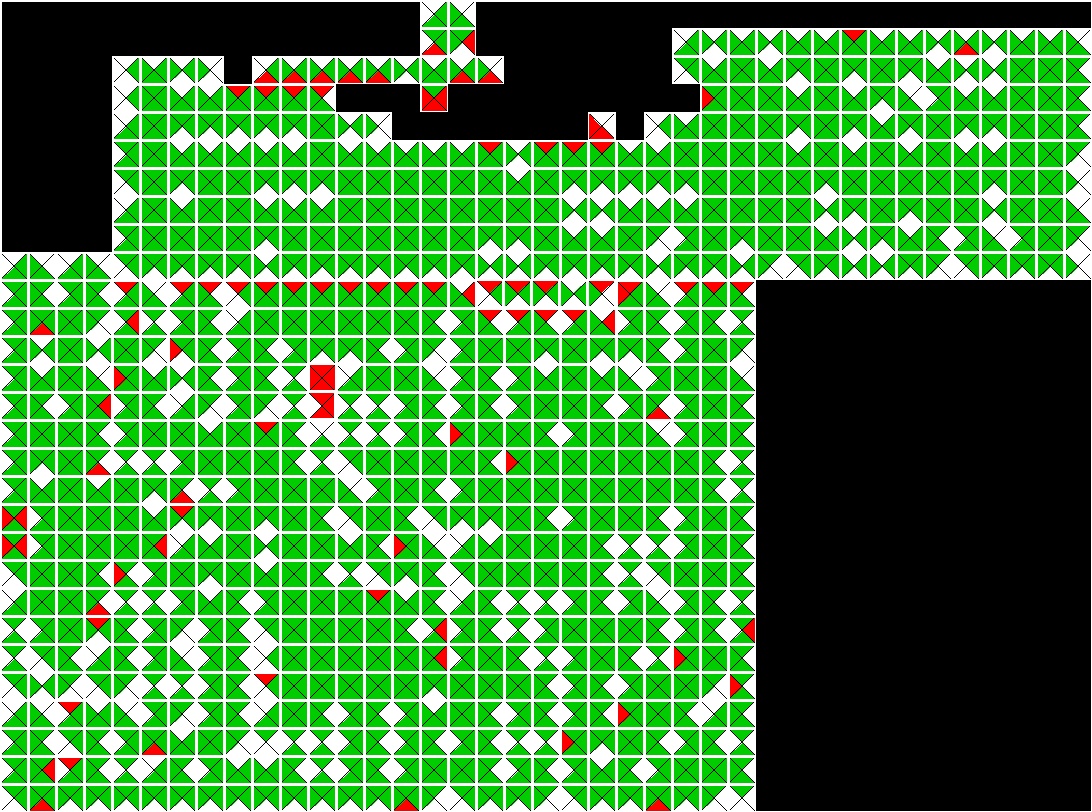
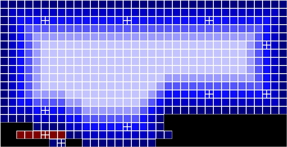
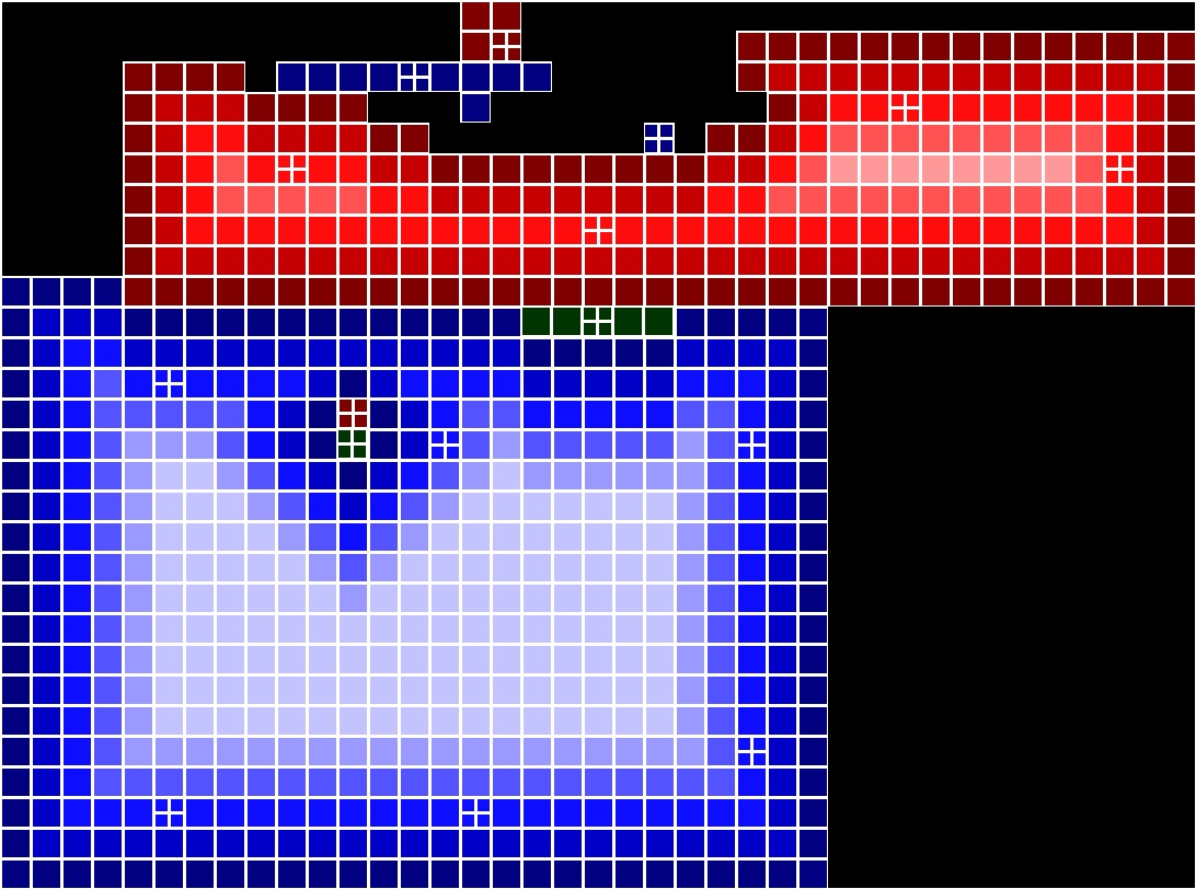
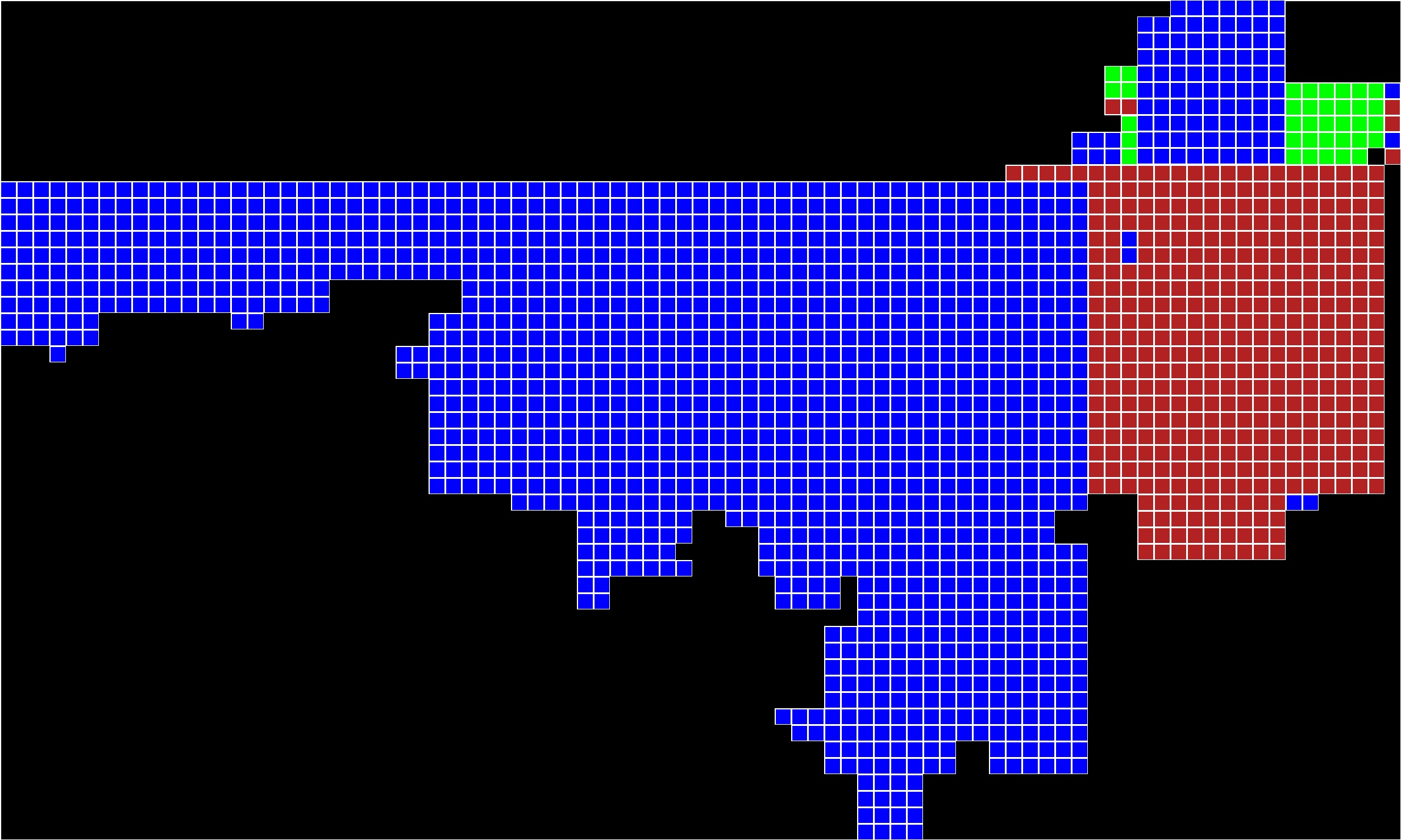
Visualizations of Piece Distance and Stitching Pieces:
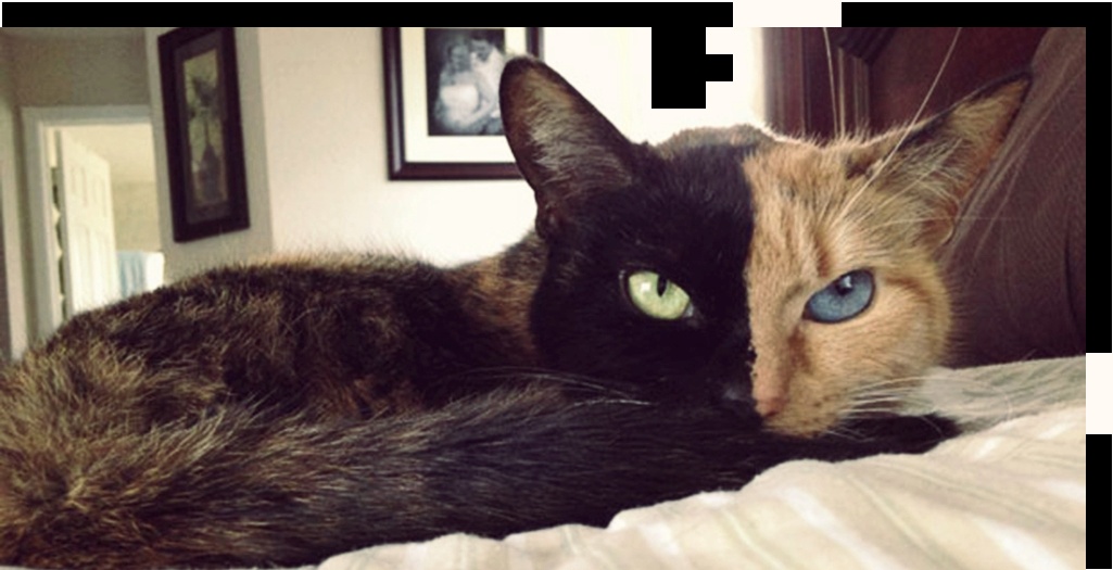
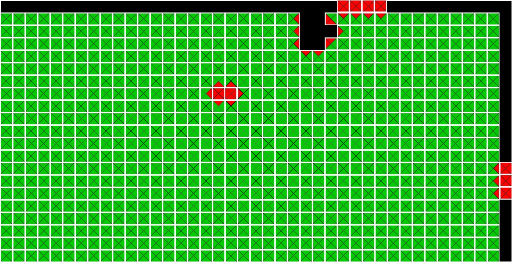
Continuing with the trend of previous weeks, I created visualizations showing the distance of each piece from an open. This is represented as a lightening gradient with the further from an open the piece is the lighter the color. Stitching pieces are indicated with a white crosshair. Below is an updated visualization from previously solved images.Input |
|
|
|
|---|---|---|---|
Solved |
 |
 |
 |
Best Buddy |
 |
 |
 |
Segmenter |
 |
 |
 |
Input |
 |
|---|
Type 1 |
Type 2 |
|
|---|---|---|
Solved |
 |
 |
Best Buddy |
 |
 |
Segmenter |
 |
 |
Input |
|
|
|---|---|---|
Solved |
 |
 |
Best Buddy |
 |
 |
Segmenter |
 |
 |
Possible improvements to the algorithm:
- Specify a minimum segment size for stitching pieces
- Specify minimum grid cell sizes
Modified Solver:
The original implementation of the solver followed the implementation of Paikin & Tal rather closely. As such, it was not implemented with multiple passes in mind. What is more, it was not written to support only partially solving a puzzle, which would be used when trying to find similarity between two neighboring segments. Work has begun on implementing this.One item that is clear is that the algorithm will need to have a better approach for spawning a new segment/board. Right now, the algorithm will spawn if the mutual compatibility drops below an arbitrarily set, predefined threshold. This can lead to huge board bloat as with the previous three puzzle problem spawning several hundred puzzles.
One problem the algorithm appears to have is that when there are a large number of pieces in a puzzle that shows relatively high uniformity, the mutual compatibility is artificially reduced meaning that boards spawn prematurely.
Summary of the Meeting on September 13, 2016:
The work for these week was divided into five primary areas, namely:- Speed-up of the mutual compatibility
- Implementation of the segmenter
- Implementation of the visualization functionality of using five colors
- Fixed bugs in the calculation of the solver accuracy
- Improving logging of the seed piece information for duplicate seed piece tracking
Segmenter:
The implementation of the segmenter for this week matches the description of the segmenter proposed last week. The only difference is that the post process cleanup is not yet performed. This will be decided after further discussion with Dr. Pollett.Five Coloring Algorithm:
The Five Color Theorem states that on a planar graph, the vertices can be colored with five colors such that no two vertices have the same color. This week, I implemented the Welsh-Powell Algorithm to assign colors to different segments in the solved image. Below is a summarized version of the algorithm:unassigned_segments = { all_segments } // Prioritize segments with most neighbors sort unassigned_segments by degree // Use a buffer to get colors sequentially C = { all valid colors} // Continue until all segments are assigned a color while |unassigned_segments| > 0 do: next_segment = unassigned_segments.next() next_color = C.next() next_segment.assign_color(next_color) // Assign the color to all other segments with no // neighbor of the same color for other_segment in unassigned_segments do: if other_segment has no neighbor with color next_color then: other_segment.assign_color(next_color) unassigned_segments.remove(other_segment)
Below is a table of two three input puzzles, the solved images, the best buddy visualizations, and the segmented images.
Input |
|
|
|
|---|---|---|---|
Solved |
|
|
|
Best Buddy |
|
|
|
Segmenter |
 |
 |
 |
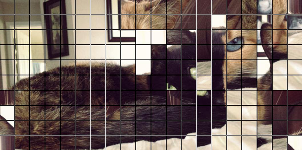
Muffins Couch Image Segmentation
Input |
|
|---|
Type 1 |
Type 2 |
|
|---|---|---|
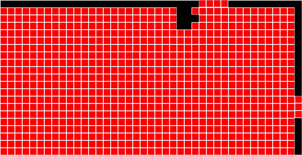
Solved |
|
|
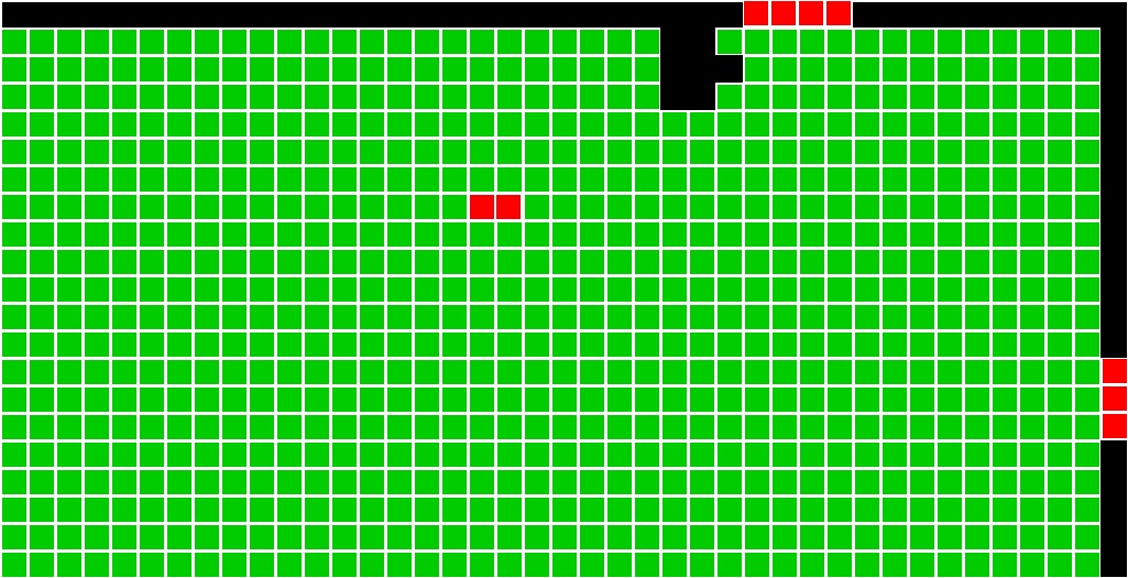
Best Buddy |
|
|
Segmented |
 |
 |
Note: In the best buddy visualization for the type 2 image, there is chaining of the main correctly assembled upper section and the incorrectly assembled lower segment. This could be fixed with the segmenter post-processing proposed previously.
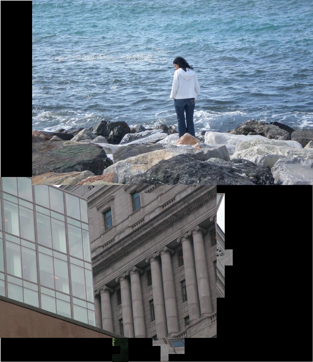
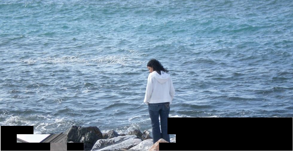
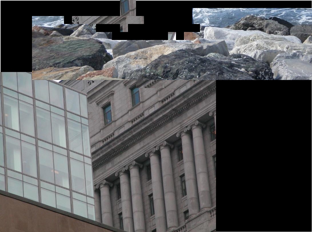
Two Image Segmentation
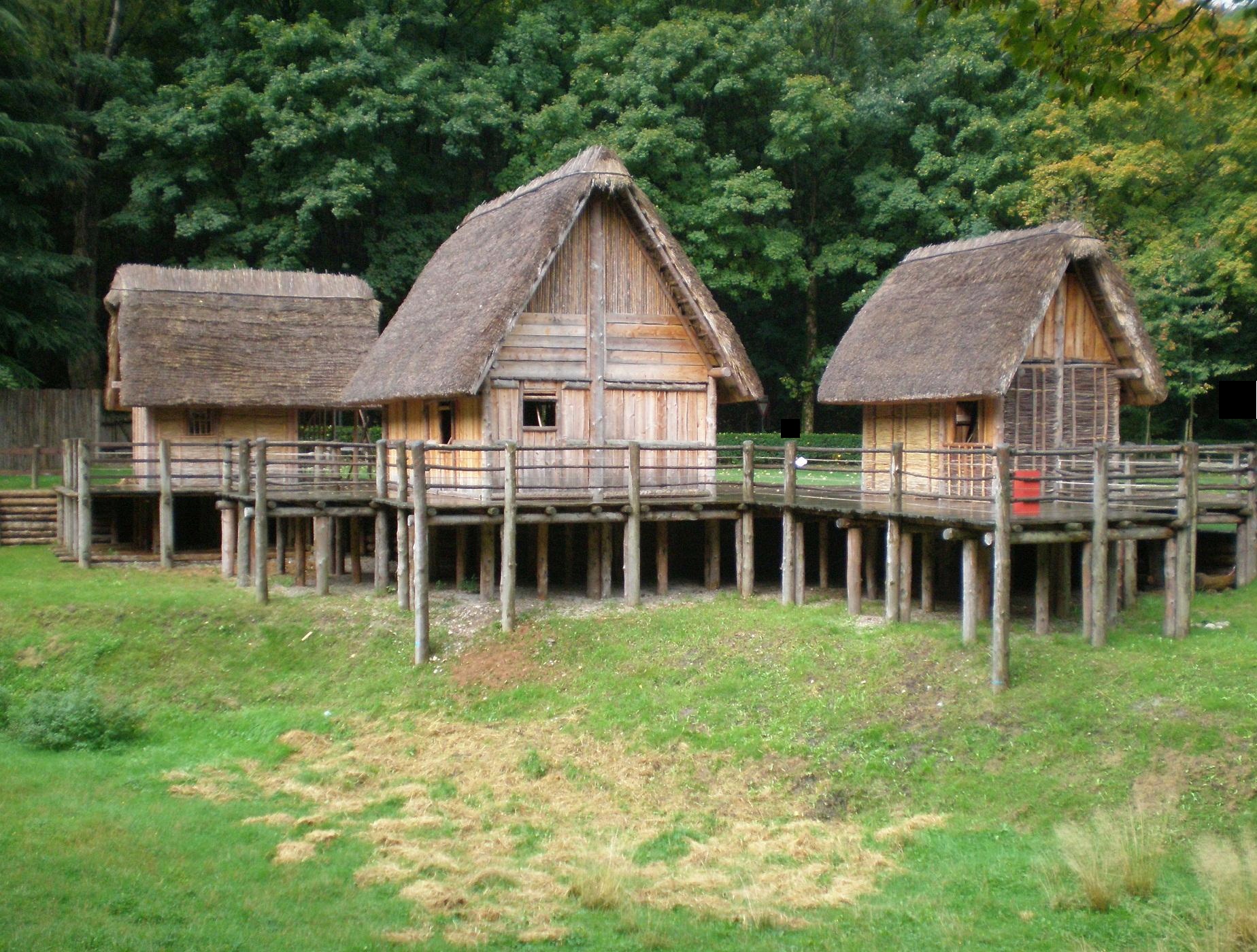
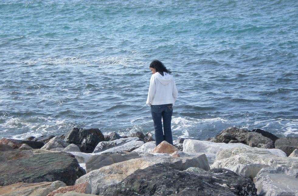
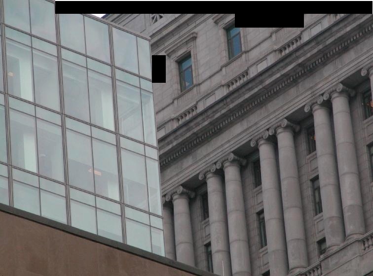
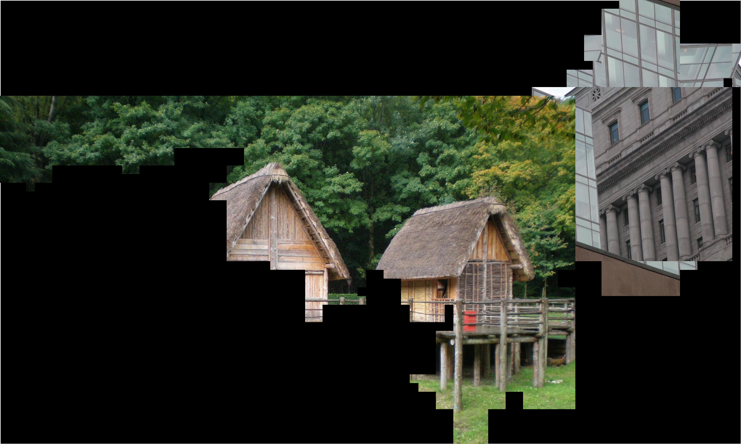
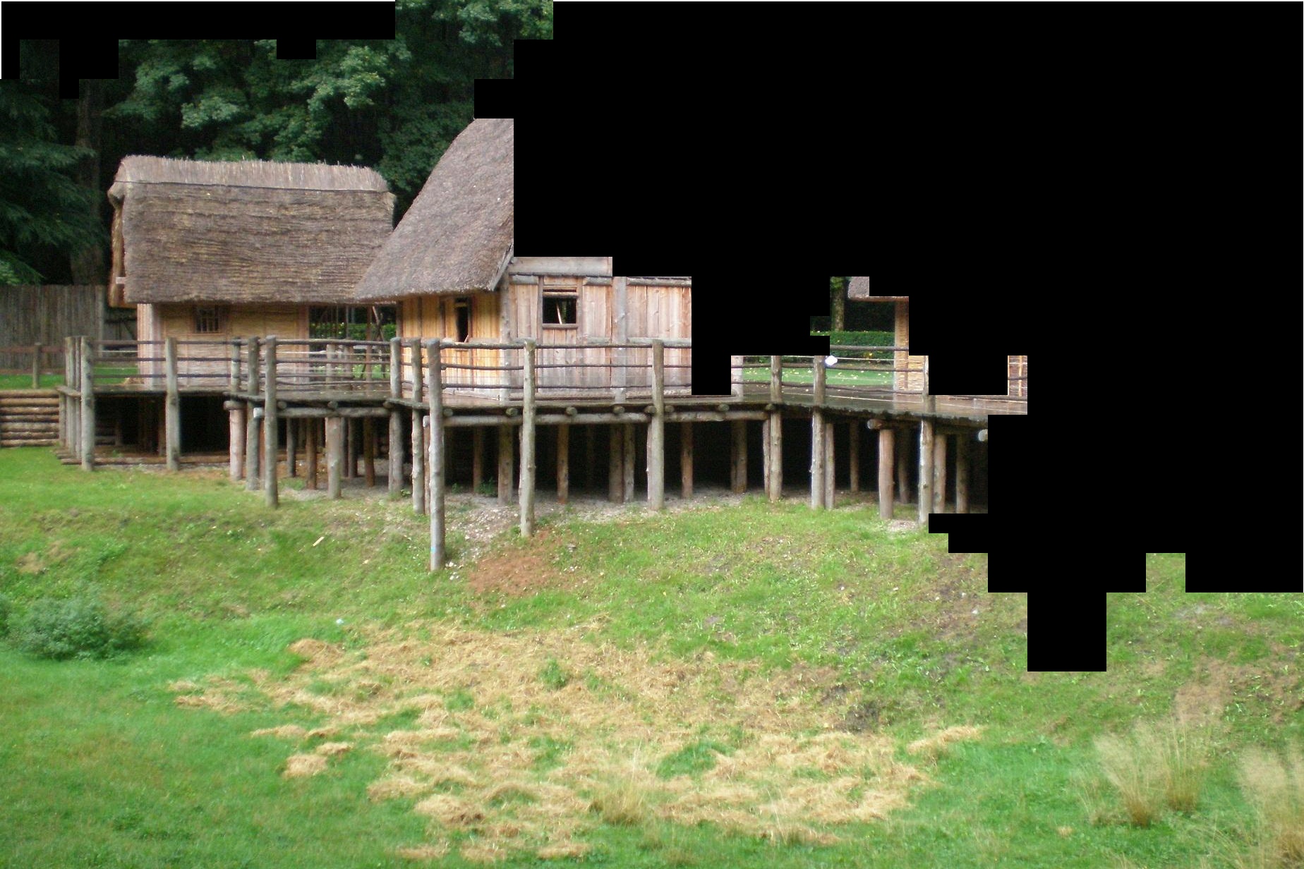
For this puzzle, the image with the two tropical style houses were removed and only the beach and building images were passed to the solver.Input |
|
|
|---|---|---|
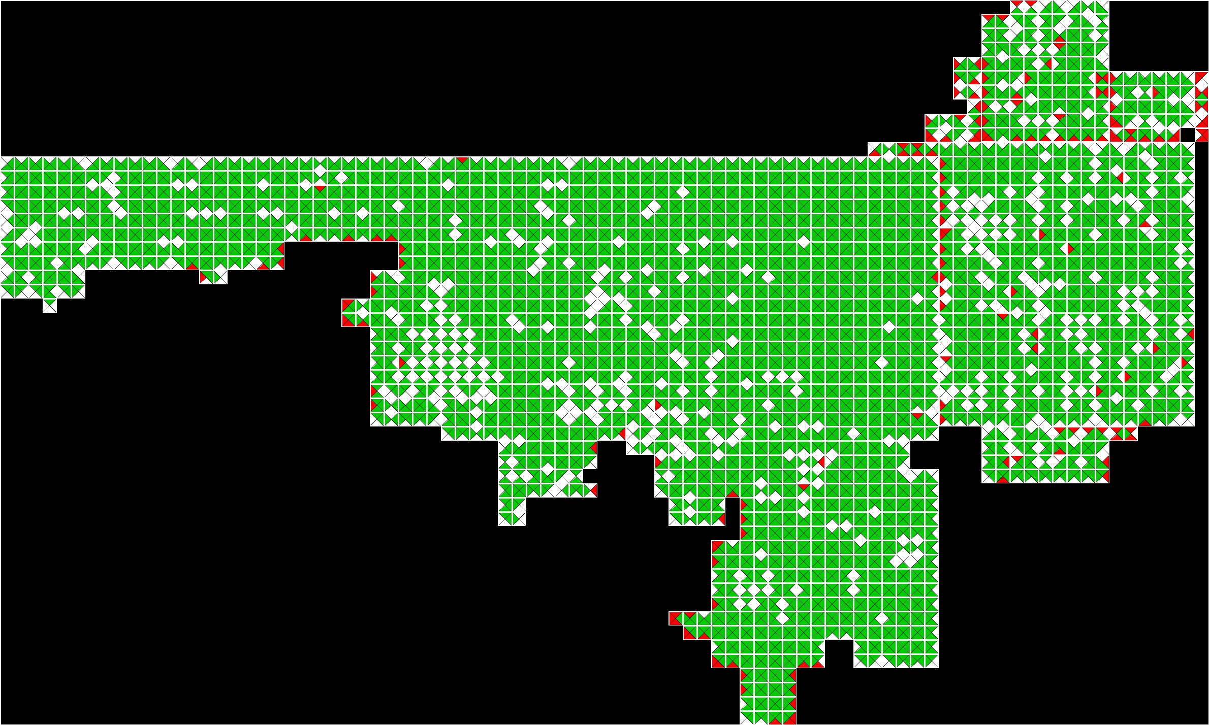
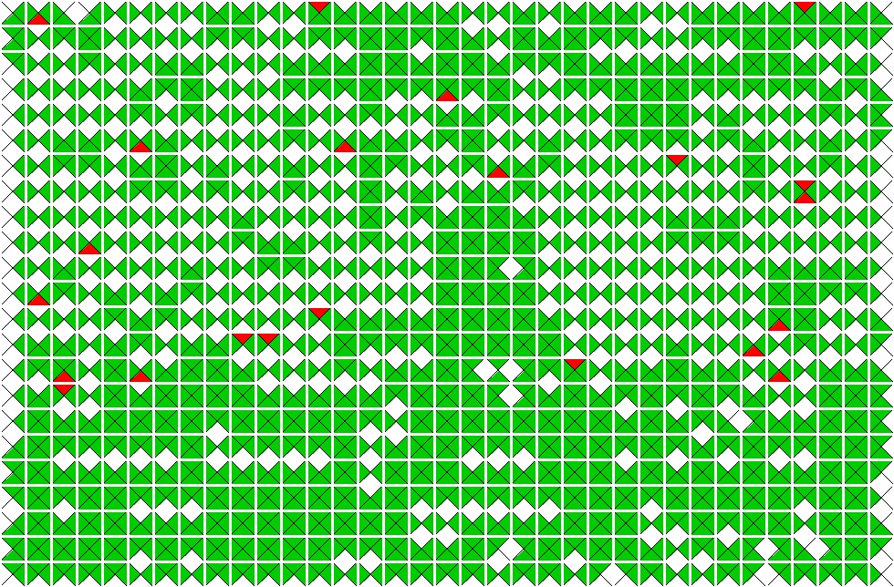
Solved |
|
|
Best Buddy |
|
|
Segmenter |
 |
 |
Logging of Seed Piece Information:
As mentioned in the last blog post, I worked extensively last week on improving the messaging logging for the program as it executes. This week, I added a feature to actually log the seed piece information so I can more easily determine if a poor seed piece was selected. For example, below is the logging that shows the solver used the seed piece from the same input puzzle for two output puzzles:Placer started Board #1 was created. Seed Piece Information for new Board #0 Original Puzzle ID: 0 Original Piece ID: 438 Original Location: (12, 18) Solver Piece ID: 438 Board #2 was created. Finding start piece candidates Finding the start pieces completed. The task "finding start pieces" took 0 min 0 sec. Seed Piece Information for new Board #1 Original Puzzle ID: 0 Original Piece ID: 582 Original Location: (16, 22) Solver Piece ID: 582
Summary of the Meeting on September 6, 2016:
For this week, I studied primarily the theoritical foundations of the solved image segmentation.Segmentation Algorithm of Pomeranz et. al.
queue  = []
numberOfSegments = 0
unassignedPieces = { allPieces }

// Greedily assign pieces to segments
while |unassignedPieces| > 0 do

	// If queue is empty, select an unassigned piece and make a new segment
	if |queue| == 0 then
		nextPiece = unassignedPieces.selectNext()
		nextPiece.assignToSegment( ++numberOfSegments )
		queue.append( nextPiece )

	// Select piece off the front of the queue
	selectedPiece = queue.pop()

	validNeighbors = selectedPiece.getValidNeighbors()
	for each neighbor in validNeighbors do
		// Skip already assigned neighbors
		if neighbor not in unassignedPieces then
			continue

		// If neighbor and selected piece are best buddies, make in the same segment
		if isBestBuddies( selectedPiece, neighbor ) then
			neighbor.assignToSegment( selectedPiece.getSegmentNumber() )
			queue.append( neighbor )
The following two subsections review some of the functions in the algorithm and discuss some of the weaknesses of the algorithm.
Description of Key Functions:
- assignToSegment: Assigns the piece to the specified segment number and removes the piece from the set of unassignedPieces.
- isBestBuddies: Returns "True" if the two specified pieces are best buddies on the specific side and "False" otherwise.
- getValidNeighbors: This function gets the top, bottom, left, and right neighbors of the specified piece (if they exist).
- getSegmentNumber: Returns the assigned segment number for a given piece.
- selectNext: This function selects the first unassigned piece starting in the upper left corner of the image and proceeds in a left-to-right, top-to-bottom fashion. As such, it searches for the left-most unassigned piece in the first row. If it does not find it, the second row is searched and so on.
Deficiencies of Pomeranz et. al.'s Algorithm:
- Poor Segment Seed Selection: The output of the segmentation algorithm is dependent on the seed piece used to start each segment. The "left-to-right, top-to-bottom" approach used by Pomeranz et. al. lacks sophistication and has room for improvement.
- Spurs and Stringing: If two pieces are best buddies, they are put into the same segement regardless of any other best buddy relationships. This can lead to "spurs" where a set of pieces that are each best buddies to one another on a single side are joined to the segment. This can also lead to "stringing" where by two unassociated segments are merged into a single segment through the previously mentioned spur.
- Boundary Pieces and Multiple Puzzles: Previous analysis on the best buddies in images preliminarily showed that the most likely places best buddies were likely to occur were around missing pieces and border pieces. This also matches the simple logical as those pieces do not naturally have a neighbor on that side and may have a tendency to form false best buddies relationships. This can be further exacerbated by the stringing issue because it may causes pieces from two different puzzles to be put into the same puzzle based off false best buddy pairings.
An Proposed Improved Segmentation Algorithm
queue = []
numberOfSegments = 0
unassignedPieces = { allPieces }

// Greedily assign pieces to segments
while |unassignedPieces| > 0 do

	// Create a new segment
	numberOfSegments++
	segment = createNewSegment( numberOfSegments )
	seedPiece = unassignedPieces.selectNext()
	queue.append( seedPiece )

	while |queue| > 0 do
		selectedPiece = queue.pop()
		selectedPiece.assignToSegmentSegment( segment )

		// Assign neighbors to the segment
		validNeighbors = selectedPiece.getValidNeighbors()
		for each neighbor in validNeighbors do
			// Skip already assigned neighbors
			if neighbor not in unassignedPieces then
				continue

			// If neighbor and selected piece are best buddies, put in same segment
			if isBestBuddies( selectedPiece, neighbor ) then
				queue.append( neighbor )

	// Post process the segment
	unassignPiecesWithWrongBestBuddies( segment, unassignedPieces )
	unassignPiecesInSpurs( segment, unassignedPieces )
	unassignedUnconnectedPieces( segment, unassignedPieces )
	// Ensure the segment is not empty after the cleanup
	if |segment| == 0 then
		 seedPiece.assignToSegment( segment )
In this essentially, a set of post processing functions are after the segment is completed. The primary goal of this function is to ensure that there is the maximum possible correctness for each segment, even at the expense of segment size. Below is the new/modified functions used in my new approach:
Description of New or Modified Key Functions:
- selectNext: Unlike Pomeranz's et. al.'s approach that lacked much sophistication in selecting the segment seed, I will borrow a bit from the approach of Paikin & Tal and prioritize segment seeds based off their level of distinctiveness.
- unassignPiecesWithWrongBestBuddies: If a piece's neighbor does not match its best buddy, then one of those pieces is removed from the segment and placed back in the set of unassigned pieces. The criteria for removal of pieces is:
- If only one of the pieces has a best buddy on the mismatching edge, then that piece is prioritized.
- The piece with the least number of correct adjacent best buddies in the segment.
- The piece that is further away from the segment seed.
- unassignPiecesInSpurs: The proposed algorithm defines a "spur" as any piece that does not have neighbors in the segment on at least two adjacent sides. All pieces in spurs are removed from the segment and placed back in the set of unassigned pieces. Completing this process may take multiple passes.
- unassignedUnconnectedPieces: This function recursively checks for any pieces that are not connected to the seedPiece via essentially a breadth first search. Any unconnected pieces are placed back in the set of unassigned pieces.
Additional Work this Week:
- Inter-piece Distance Calculation Spped-up: As previousl.y mentioned, one of the most time consuming aspects of Paikin and Tal's algorithm is the interpiece distance calculation. In the latest code, I have modified the implementation to now use multiple process to parallelize the computation. This approach is multi-process and not multi-threaded due to the issues associated with Python's GIL. As an example of the speed-up, a calculation that used to take 13min 14s now takes 5min 16s (an ~60% speed-up). With some additional minor changes, more sppedup is expected.
- Logging: In previous versions of the program, the implementation of loggin was to put it mildly poorly implemented. All mesages were printed to the console. No log messages were assigned priorities (e.g. "info", "debug", "critical", etc.). This has totally be rewritten and is now much more flexible and scalable.
Questions for Dr. Pollett:
- Segment Coloring Algorithm: Being able to visualize the segmentation output would be very helpful. The most challenging aspect of this is how best to color the visualization. What approach could be taken to do this as simply as possible?
- Access to CSS Files: When updating the blog, it would be useful to make custom CSS file entries to simplify some of the formatting. Is this possible with the existing website template?
Summary of the Meeting on April 26, 2016:
Activities for this week focused on three primary tasks:- Best Buddy Accuracy Tool for Original (i.e. Unsolved) Images: In my previous implementation, best buddy accuracy was calculated in real time as the solver was being run. This meant that I had no way to calculate the best buddy accuracy on an unsolved image. This week, I created a best buddy unanalyzer for original images. This tool also provides more advanced statistics on the best buddy accuracy.
- Best Buddy Placer: Last week, I proposed placing using best buddies as highest priority. I made a quick implementation of this feature, which provided mixed results.
- Documentation Builder: Throughout the development process, I made an effort to write meaningful Python docstring comments while I was developing. I was not previously able to get Sphinx working. After some efforts this weekend, it is now working.
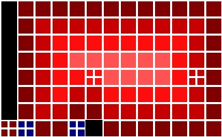
Best Buddy Accuracy for Input Images:
As mentioned previously, I added support for determining the best buddy accuracy of input images. When determining the accuracy, I determine the following statistics:- Total Number of Best Buddies: Some images have lower best buddy density. This will capture the best buddy density of the input image.
- Density This is a ratio of the total number of best buddies versus the number of possible best buddies (i.e. number of pieces multiplied by the number of sides for each piece).
- Total Number of Interior Best Buddies: An interior side in an puzzle is any side that has an neighbor next to it. This calculates the total number of interior best buddies (right or wrong).
- Number of Wrong Interior Best Buddies: A wrong interior best buddy is any interior best buddy where the best buddy is not the piece's actual neighbor.
- Number of Wrong Exterior Best Buddies: Any best buddy on the exterior (i.e. either on the outer edge of the puzzle or next to a missing piece) is guaranteed to be wrong. This statistic tracks the number such pieces separately.
- Accuracy Best buddy accuracy is defined as 1 minus the ratio of wrong best buddies (i.e. sum of exterior and interior) over the total number of best buddies.
- Advanced Statistics on Per Piece Best Buddy Accuracy versus Number of Pieces: A piece in the puzzle can have as many best buddies as it has sides (i.e. up to four best buddies for a four sided piece). This statistic is stored in a 3D matrix which represents the number of best buddies (from 0 to number of sides) versus number of wrong interior best buddies versus number of wrong exterior best buddies.
Original Image |
Best Buddy Accuracy Visualization |
|---|---|
 |
 |
Some of the best buddy statistics for this image are:
- Number of Pieces: 289
- Total Number of Best Buddies: 488
- Best Buddy Density: 42%
- Accuracy: 94.67%
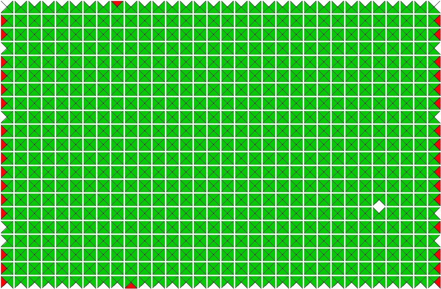
Best Buddy Placer:
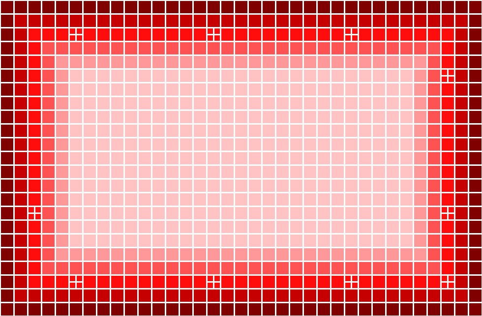
As discussed in the blog last week, one idea for an improved placer is to prioritize placing a piece based off its number of best buddies rather than placing off a single side. That would allow for information from more than a single side to be used at a time. This placer had mixed results. The first image below is the standard image of Muffins I use. I have included with it the best buddy accuracy visualization as well.Original Image |
Best Buddy Accuracy Visualization |
|---|---|
 |
 |
Paikin & Tal Placer |
Best Buddy Placer |
 |
 |
The best buddy statistics for Muffin's image are:
- Number of Pieces: 70
- Total Number of Best Buddies: 206
- Best Buddy Density: 73%
- Accuracy: 97.09%
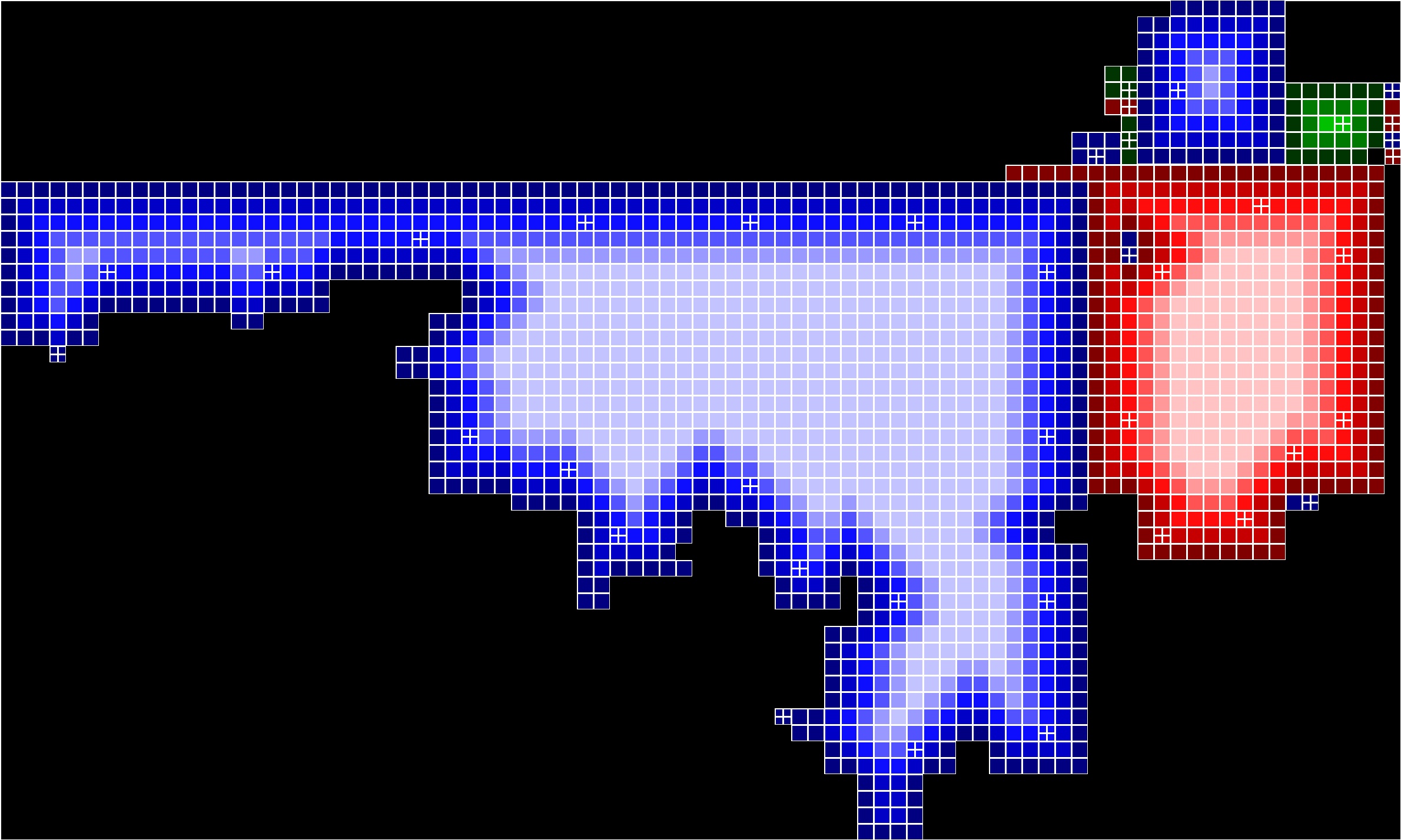
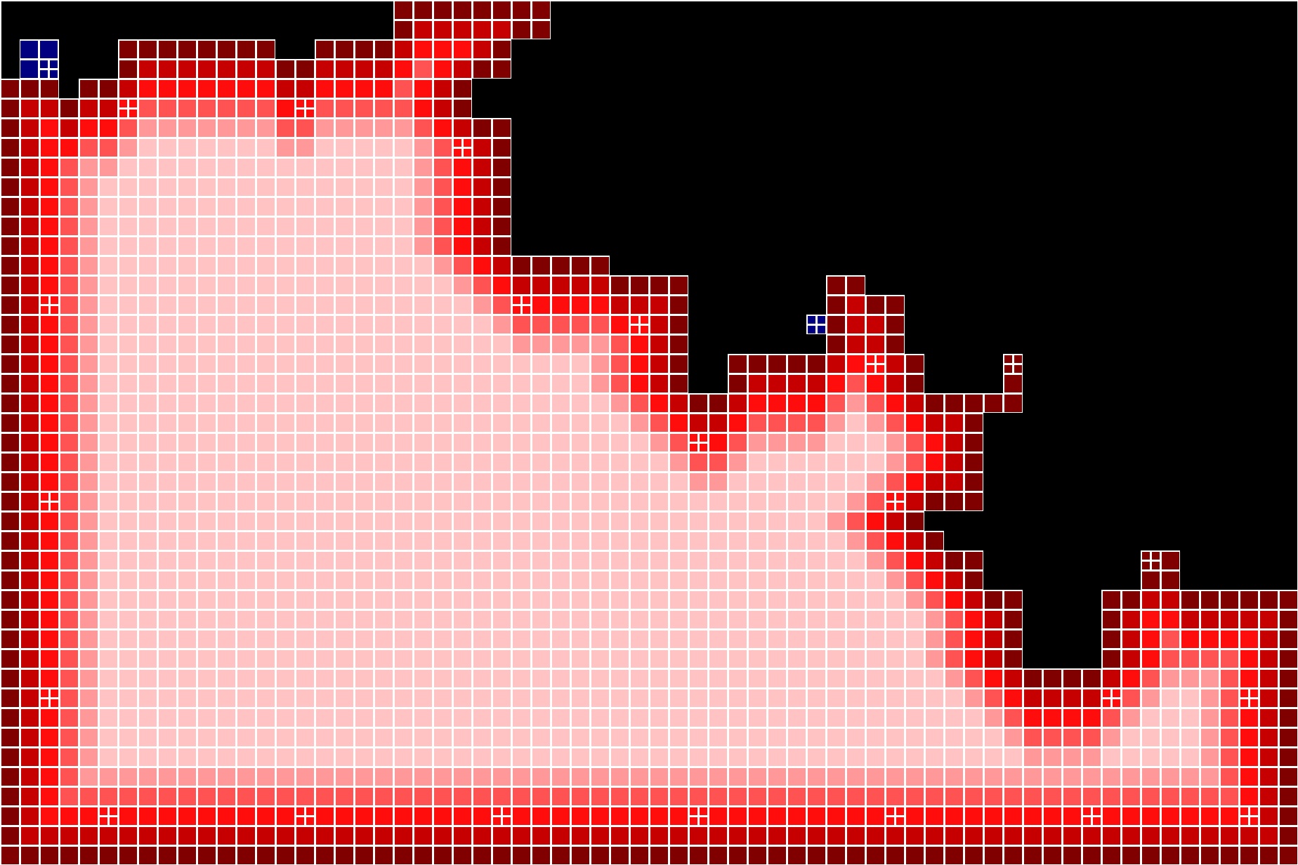
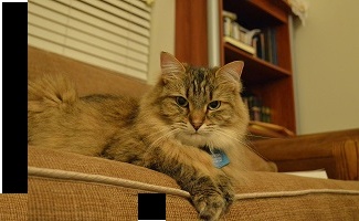
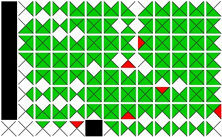
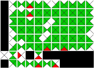
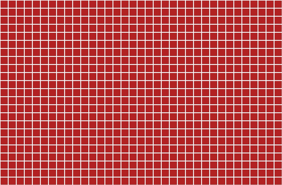
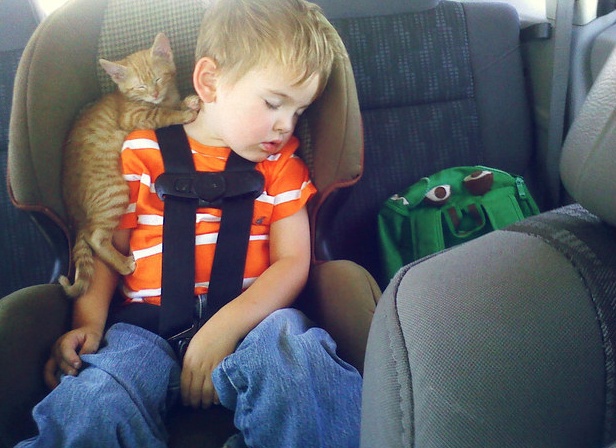
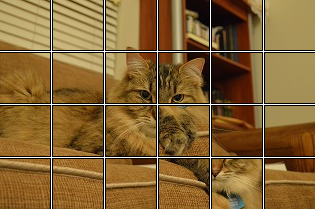
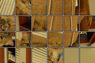
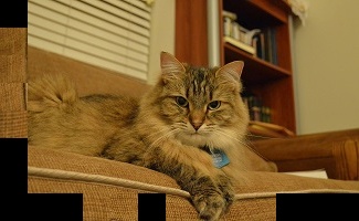
In contrast, when I used the best buddy solver on the cat with the boy image, I performed slightly worse. Below are the images. The incorrectly placed piece is shown in the best buddies visualization with a blue border.
Original Image |
Best Buddy Accuracy Visualization |
|---|---|
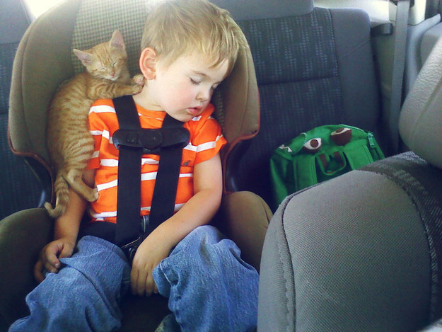 |
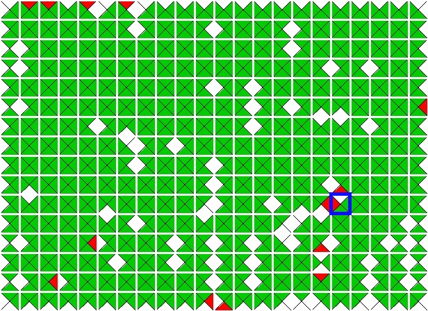 |
Paikin & Tal Placer |
Best Buddy Placer |
 |
 |
The best buddy statistics for the boy with the cat are:
- Number of Pieces: 352
- Total Number of Best Buddies: 121
- Best Buddy Density: 86%
- Accuracy: 97.09%
Items Meriting Future Thought/Work:
Below are items meriting more work or thought. It includes known bugs.- Direct Accuracy Not Considering Missing Pieces: In my current implementation of calculating direct accuracy, I do not consider missing pieces properly when calculating the accuracy. This is a bug that needs to be fixed.
- Histogram of Pieces by Number of Best Buddies: In a given puzzle, the more best buddies the piece has, the more likely it is that it will be easily solvable. For example, a piece with 0 best buddies is really hard to solve. This needs to be more closely studied.
Summary of the Meeting on April 19, 2016:
Before going in depth on each of the activities from this week, I want to give a quick summary of each:- Implementation Best Buddy Estimation Metric: In the literature, the number of correct best buddies is the only metric that has shown substantial promise as an estimation metric for solved results that does not rely on the ground base image. This feature was implemented in my solved and went through extensive testing. The way the code is implemented, BB is found in real time.
- Results Data Visualization: Previously, I had no effective way to visualize the placement results other than looking for errors in the solved image. I added a new visualization component as well.
- Handling of Ties for Second Place Distance: Paikin & Tal specify that the second best distance is used to determine the asymmetric compatibility between pieces. I modified my implementation around this and am getting much better results on computer generated images like the duck.
- Using the Vertical Change for Calculating Inter-Piece Distance: One of the ideas Dr. Pollett and I previously discussed was using not only horizontal change to calculate interpiece distance but also vertical pixel to pixel changes.
- Heap Cleanup: To improve placer performance, periodically clean the placement heap.
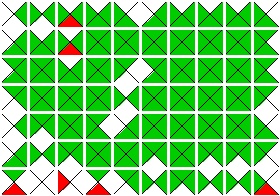
Best Buddies Estimation Metric:
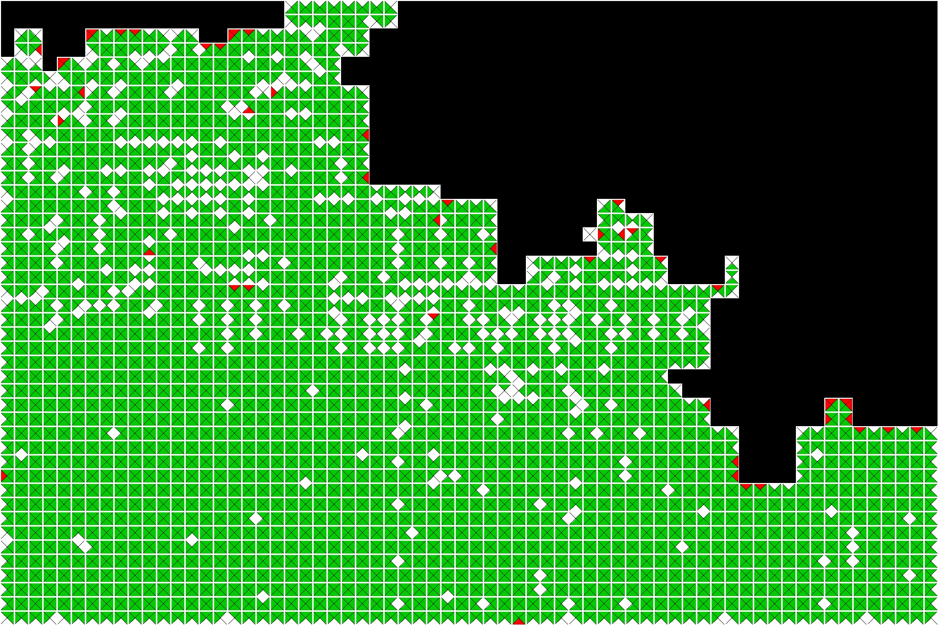
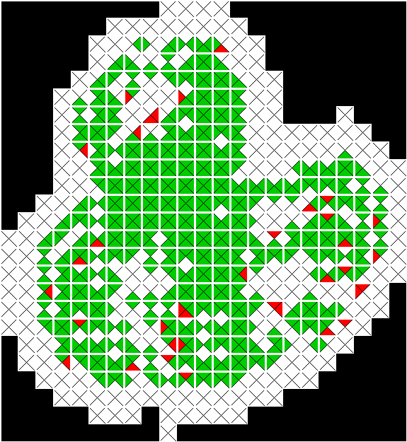
This was the area with the most progress this week. As mentioned previously, best buddies is a estimation metric for determining the quality of a solved image either at the end of placement or during placement in real time. A "correct" best buddy are when two best buddies that are placed adjacent to one another. In contrast, a "wrong" best buddy is when two best buddies are not placed next to one another. In the literature, this is as far as best buddy error classification goes. I propose instead classifying "wrong" best buddies" into two separate categories namely:- Border "Wrong" Best Buddies: These are best buddies that are not adjacent but are on the border of an image either due to missing pieces or due to them being along the edge of an image. These are much more common in actual images since they have no natural pair. What is more, these are of only limited utility when understanding the quality of an image.
- Inner "Wrong" Best Buddies: These are best buddies that are placed next to an actual piece (i.e. not on an edge). These are generally far fewer in a puzzle and generally more meaningful.
Solved Image |
Best Buddy Accuracy Visualization |
|---|---|
 |
 |
To date, I have yet to find a single puzzle piece that had more wrong best buddies than right best buddies.
An Improved Solver:
Paikin and Tal place best buddies into a pool and then place from that pool the piece that has the best match. This can lead to some poor placements in particular because the solver is greedy.In the end, Paikin & Tal want to prioritize placing the piece with the highest confidence first. However, using only one side to do that is not going to always lead to very good results. New placement priority:
- Priority #1: Select for placement the piece with the highest number of best buddies at any location. Break ties based off the piece with the highest mutual compatibility.
- Priority #2: If no piece has a best buddy at any location, place the piece from the best buddy pool with the highest mutual compatibility with any piece.
- Priority #3: Recalculate mutual compatibility and pick the piece with the best mutual compatibility.
Results Visualization Tools:
As mentioned previously, my ability to visually tell the quality of placement was limited to reviewing the outputted image. This is a poor approach in particular when many pieces may appear similar to one another. To remedy this problem, I made visualization tools that show the quality of placement results. Excluding the best buddy visualization tool described previously, three additional visualization tools were created namely:- Standard Direct Accuracy Visualizer
- Modified Direct Accuracy Visualizer
- Neighbor Accuracy Visualizer
Standard and Modified Direct Accuracy Visualizer
When the accuracy of piece is determined via the "direct accuracy" approach, it falls into one of four categories:- Wrong Puzzle: The piece is placed with pieces that are predominantly from a different puzzle
- Wrong Location: The piece is placed with pieces from its original puzzle but in the wrong location.
- Wrong Rotation: The piece is placed in the right location but with the wrong rotation (i.e. not 0 degrees).
- Correct Location: The piece is placed with no rotation, in its correct location, and in a solved puzzle where pieces from its puzzle are the most common.
Wrong |
Wrong |
Wrong |
Correct |
|---|---|---|---|
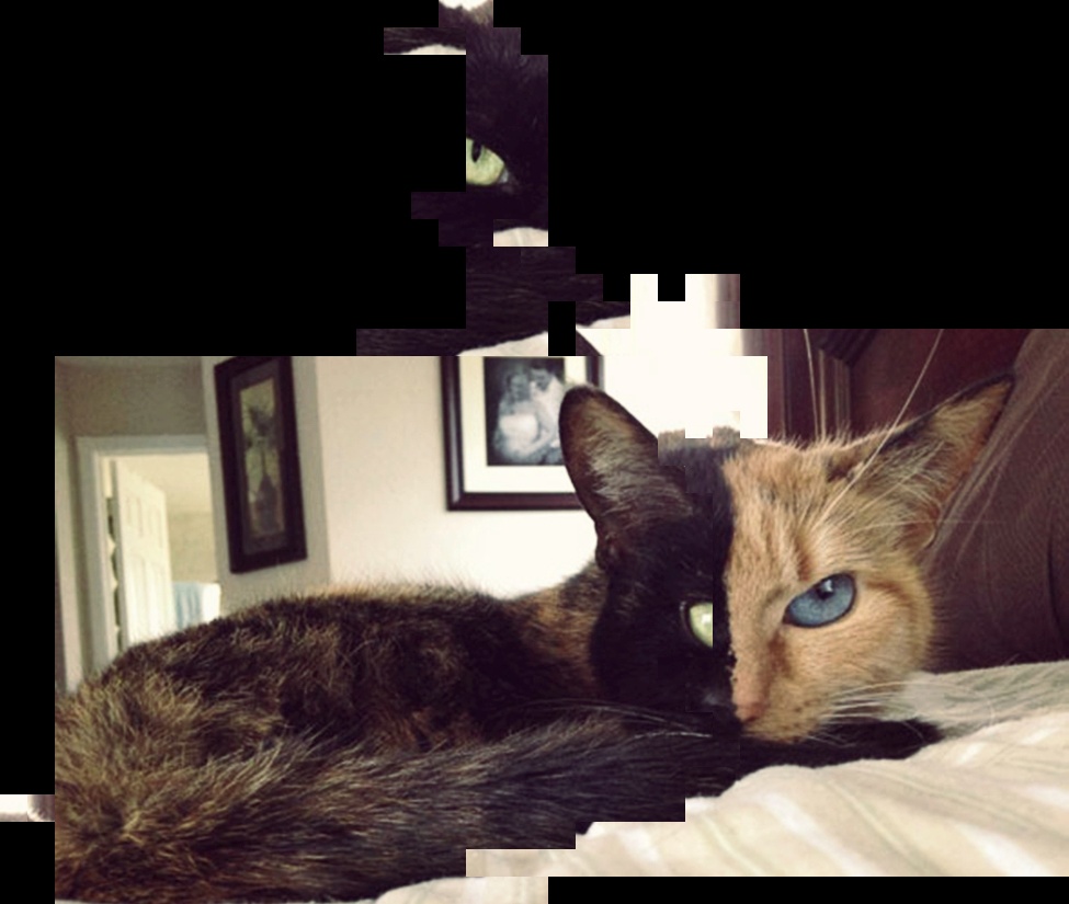
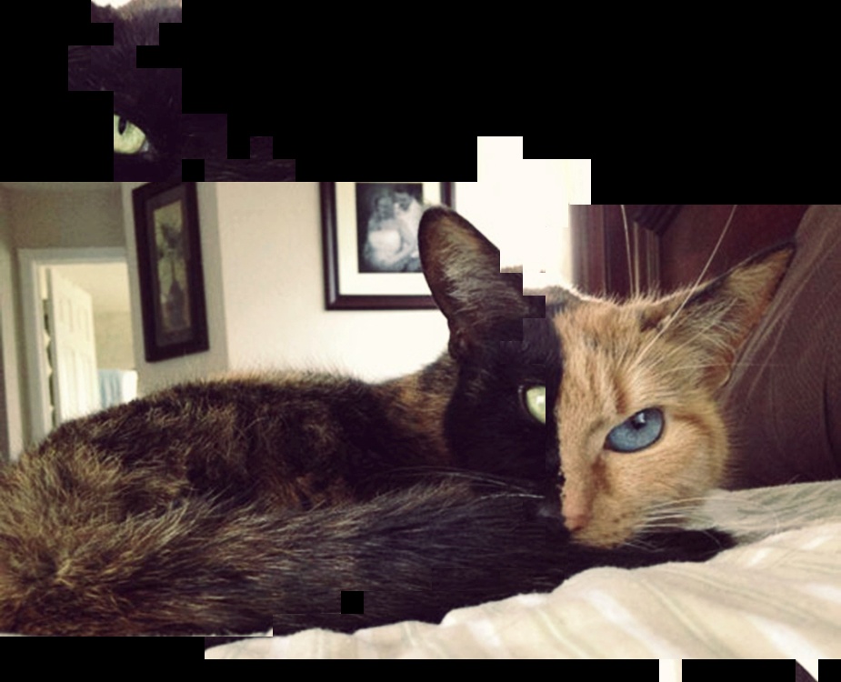
Below are the standard and shiftable direct accuracy visualizations for the two-faced cat image solved as type 2 puzzle.
Solved |
 |
|---|---|
Standard |
 |
Shiftable |
 |
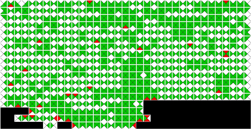
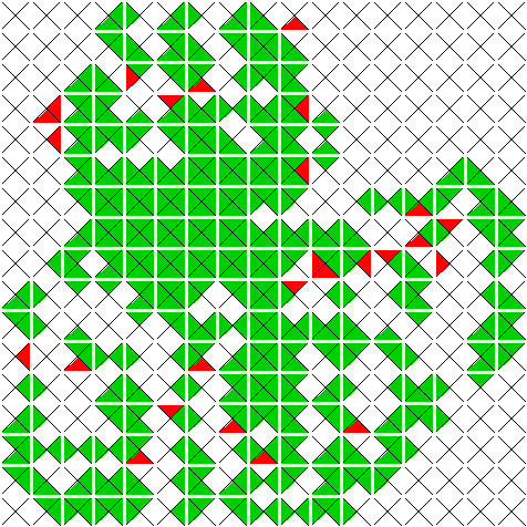
Neighbor Accuracy Visualizer:
Unlike direct accuracy where a single correct/wrong designation is given to each piece, each piece is given multiple neighbor accuracy classifications (i.e. one for each side). Hence, its case is much closer to the approach needed to visualize best buddy accuracy.Each puzzle piece is assigned to one of three accuracy categories namely:
- Wrong Puzzle: The piece is placed adjacent to a piece from a different puzzle. What is more, this other puzzle does not have the most pieces in the solved puzzle
- Wrong Neighbor: The piece is not next to the same piece's side as in the original image.
- Correct Neighbor: The side of the piece is assigned to the same side of its neighbor piece that it was in the original puzzle.
Wrong |
Wrong |
Correct |
|---|---|---|
Below is the neighbor accuracy visualizations for the two-faced cat image solved as type 2 puzzle.
Neighbor |
 |
|---|
Improvements for Computer Generated Images:
Due to variations in the environment as well as in the camera, it is unlikely to get areas in photographs that the same RBG value over a large number of pixels. That is possible however in computer generated and computer manipulated images. We saw this issue both in the Che Guevarra image and in the Duck image. Using a very simple code modification and by disallowing multiple best buddies, I was able to drastically improve my performance on the duck image. Below is my original code for determining the distance between two pieces. Note that if the piece to piece distance was 0, I always set the asymmetric distance to 0, even if the second best distance was "0". In other words, I was prioritizing 0 distance over the undefined case (i.e. divide by 0). That was causing all sorts of problems.Original Code |
Improved Code |
|---|---|
|
|
When I made the change as shown on the left above, my performance on the duck image improved dramatically as shown below. Note this is solved as a type 1 puzzle.
Previous Duck Result |
Latest Duck Result |
|---|---|
 |
 |
Below is a visualization of the solved image's neighbor and best buddy accuracies.
Shiftable Direct Accuracy |
Neighbor Accuracy |
Best Buddy Accuracy |
|---|---|---|
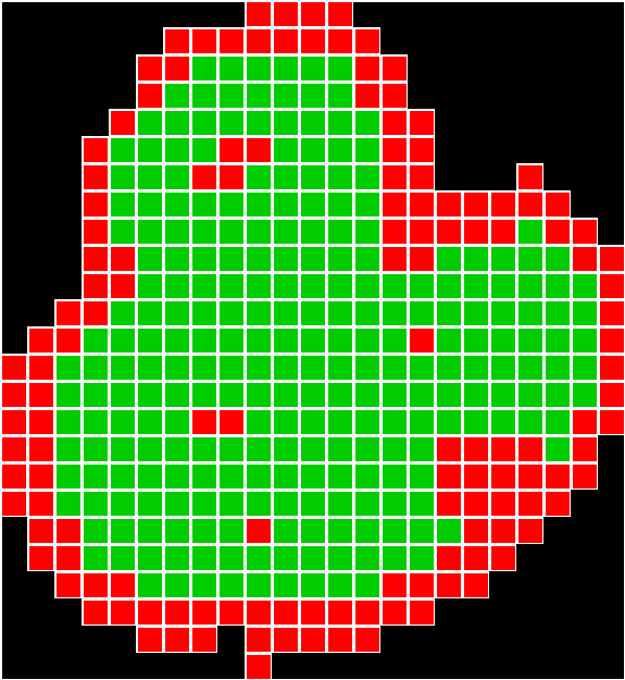 |
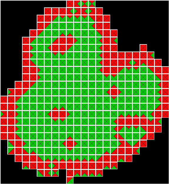 |
 |
Using Vertical Pixel Difference Information in Calculation Inter-Piece Distance:
This was an idea that originated from a meeting between Dr. Pollett and myself a few weeks back. It was intended to find pixels of increased interested by using vertical changes in addition to horizontal changes in value. The initial experiments this week were rather crude. However, it merits more consideration once a better approach is devised.Placed Speed-up Via Heap Cleanup:
A max heap is used to store the candidates for placing. As pieces are placed, new elements are added to the heap. As such, the pairings that are very poor sink to the bottom of the heap and are never removed even if that pairing becomes impossible because a piece was placed or because a slot became filled. To speed up placement, I now added a feature to periodically clean the heap. The algorithm for cleaning is the heap size must exceed at least a million elements and it must be at least 100 placements before teh last heap cleaning. Tweaking of these parameters would be required to improve the performance gain from this approach.Summary of the Meeting on April 12, 2016:
In Cho et. al., two puzzle result accuracy measures were proposed, namely "direct accuracy" and "neighbor accuracy." Direct accuracy is defined as the number of pieces placed in the correct location with respect to the original image. In simplified versions of the jigsaw puzzle problem, this definition has sufficient clarity. However, it runs into issues in the following cases:- Multiple Puzzles: When there are multiple puzzles being solved simultaneously, this metric does not define how to handle the case where there may be pieces from multiple puzzles in the solved image. What is more, when solving multiple puzzles, some of the pieces from the original image may not be present in the "most compatible" solved image.
- Non-Fixed Puzzle Boundaries: Direct accuracy is known to be susceptible to shifts in the input image. This sensitivity is exacerbated the puzzle size is treated as unknown as a single misplaced piece can cause the direct accuracy to become zero.
EDAS
To address these limitations when solving multiple puzzles with non-fixed puzzle sizes, I proposed a new metric known as the "Enhanced Direct Accuracy Score" (EDAS) that is defined as:`EDAS_i = \max_{s_j \in S}((c_(ij))/(n_i + \sum_{k \ne i}(m_(kj))))`
given:
- `P` - Set of all input (i.e. original) puzzles
- `p_i` - `i^(th)` input puzzle in the set `P`
- `n_i` - Number of pieces in puzzle `p_i`
- `S` - Set of all solved puzzles (where `|S| <= |P|`)
- `s_j` - `j^(th)` input puzzle in the set `S`
- `m_(kj)` - Number of pieces from input puzzle `p_k` that are in solved puzzle `s_j`
- `c_(kj)` - Number of pieces from input puzzle `p_k` that are placed in their correct location in `s_j` (where `0<=c_(kj)<=m_(kj)`)
EDAS addresses the issue of multiple puzzles by considering both pieces from other input puzzles as well as pieces from puzzles other than the puzzle of interest. An additional benefit of EDAS is that when solving a single puzzle with a known fixed size, EDAS and the direct accuracy are equivalent.
One additional important note is that EDAS is score and not a measure of accuracy. While its value is bounded between 0 and 1 (inclusive), it is not specifically defined as the number of correct placements divided by the total number of placements (since `(n_i + \sum_{k \ne i}m_(kj))` may be greater than the number of pieces in the solved puzzle `p_j`).
S-EDAS
While EDAS effectively defines how to account for multiple puzzles in the accuracy score, it does not address the issue of non-fixed puzzle boundaries. To handle that, we propose the Shiftable Enhanced Direct Accuracy Score (S-EDAS). The way this approach differs from EDAS is that EDAS always considered the top-left puzzle piece location as the reference point when determining the correct placement of pieces. In contrast, S-EDAS allows that reference location to shift with the maximum shifting being the minimum Manhattan distance between the upper left corner of the image and any placed piece.It is important to note that S-EDAS should not be considered a replacement for EDAS. Rather, it is supplemental as high direct accuracy score indicates that the solved image has no shifting while same conclusion can not necessarily be drawn from a high S-EDAS score (for example the image with a high S-EDAS score may be shifted). Instead S-EDAS is intended to remedy cases both EDAS and direct accuracy are misleadingly punitive. It is also true though that as a puzzle solution improves that the both EDAS and S-EDAS should increase with both being 1 for a perfectly solved image.
ENAS
The second metric for measuring the quality of a solved puzzle is "neighbor accuracy" which is the "fraction of the four neighbor nodes that that are assigned the correct [piece] (i.e. [pieces] that were adjacent in the original image)." While neighbor accuracy is more immune than direct accuracy to shifts and non-fixed puzzle borders, it is still is not designed to handle solving multiple puzzles. Due to this, we propose the Enhanced Neighbor Accuracy Score (ENAS) defined as:`ENAS_i = \max_{s_j \in S}((a_(ij))/(q*(n_i + \sum_{k \ne i}(m_(kj)))))`
given:
- `P` - Set of all input (i.e. original) puzzles
- `p_i` - `i^(th)` input puzzle in the set `P`
- `n_i` - Number of pieces in puzzle `p_i`
- `S` - Set of all solved puzzles (where `|S| <= |P|`)
- `s_j` - `j^(th)` input puzzle in the set `S`
- `m_(kj)` - Number of pieces from input puzzle `p_k` that are in solved puzzle `s_j`
- `a_(kj)` - Number of sides of each piece from input puzzle `p_i` that is adjacent to the same neighbor side as in the original image.
- `q` - Number of sides for each piece (e.g. 4).
Summary of the Meeting on April 5, 2016:
There was no meeting last week due to San Jose State's Spring Break. Over the last two weeks, I have been working on refining and improving my implementation of the Paikin & Tal solver. Significant accomplishments include:- Placer Speedup: For a board of a few hundred pieces, the placing stage would take several minutes which is much longer than it should. In the version uploaded to fulfill the requirements of deliverable #3, the implementation uses a heap to manage the pairings of best buddy pool to open locations. Additional speed-up may be possible if I periodically clean the pool, but that remains to be investigated.
- Optional Board Dimensions Attribute: In earlier attempts to solve the Jigsaw puzzle problem, the algorithm was supplied with the size of the board which constrained the placement. This is now only an optional feature in Paikin & Tal's implementation. I have implemented this feature.
- Support for Multiple Puzzles: In my earlier blog posting two weeks ago, my implementation only supported a single puzzle. This has been enhanced.
- Compatibility Recalculator: One of the methods for measuring the accuracy of a placement is the number of correct neighbors versus the total number of piece neighbors. Support for this feature will comprise deliverable #4 for my CS297.
- Laying the Foundation for the Neighbor Based Accuracy Method: One of the methods for measuring the accuracy of a placement is the number of correct neighbors versus the total number of piece neighbors. Support for this feature will comprise deliverable #4 as enumerated in my CS297 proposal.
- General Bug Fixes: Overall the solver does a good job on most images. With that said, it does not mean the code is without bugs. I am fixing bugs as I find them. I expect this to be a long, ongoing process.
Original Image |
Solved Image |
|
|---|---|---|
Image #1: (672 Pieces) |
 |
|
Image #2: (540 Pieces) |
 |
 |
Based off my experiments with Paikin and Tal's tool, below are what I see as the weak points in the algorithm:
- Images with Significant Areas of Low Texture Space: This weakness is mentioned by Paikin & and Tal as well. When there is low density, the tool does poorly.
- Improved Picking of the Starting Piece: The start piece has a huge impact on the performance of the algorithm since it is greedy. Perhaps use a depth search to find the area of connected components.
- Spawning New Boards: Paikin & Tal use a fixed value as the threshold to spawn new boards. This approach is prone to error as on large puzzles with multiple possible starting piece candidates, you may spwan two boards with pieces from the same source image.
- Lack of Best Buddies: In earlier attempts to solve the Jigsaw puzzle problem, the algorithm was supplied with the size of the board which constrained the placement. This is now only an optional feature in Paikin & Tal's implementation. I have implemented this feature.
- Smaller Puzzle Piece Size: The standard puzzle piece size for a long time has been 28 pixels by 28 pixels. I have experimented with pieces 25 pixels by 25 pixels (about 20% smaller) and the accuracy goes down. This would point to the need for an improved distance metric.
- Clearing the Best Buddy Pool?: When a new board is spawned, all pieces in the best buddy pool are cleared. I am not sure this is the best approach given the issue mentioned previously with the recalculation approach (whcih will be needed for any pieces in that puzzle.
- Multithreading: The majority of the algorithms runtime is spent calculating the interpiece distances. Since most of the calculations are independent, it could be made multithreaded in a relatively straightforward manner.
- Prohibitive Interpiece Distances: One of the speed-ups Paikin & Tal propose is to skip calculating the interpiece distance for pieces when the distance between the average pixel weight is above a certain threshold. This should greatly speed up execution if implemented.
- Coloring of incorrectly placed Pieces: It will be useful to visualize incorrectly placed pieces. A feature will be needed to support this approach.
Summary of the Meeting on March 22, 2016:
Significant progress on the Paikin & Tal solver. A few notes on the accomplishments:- Dataset Acquisition: Most of the premier papers that work on the jigsaw puzzle problem reference a handful of datasets. Examples of datasets include: Cho et. al. (2010), McGill, and the Ben-Gurion University dataset from Sholomon et. al.. I found some of the datasets located on the website for Sholomon et. al.'s work. This blog post includes work from some of the images in the dataset.
- Testing Architecture: To ensure the correctness of the work, I implemented a testing architecture for both the puzzle importer and the inter-piece distance modules. I also created a toy board to use to verify the proper implementation of the project. Both are very useful for finding bugs.
- Mutual Compatibility and Asymmetric Compatibility Calculators: I rewrote part of the implementation from last week around asymmetric distance to make the storage more streamlined and the computation of the respective distances faster. Using this modified approach, it calculating asymmetric distance was made more efficient.
- Starting Piece Calculator: This is now verified working. It may need some efficiency improvements, but all in all, it is working sufficiently well for proof of concept.
- Greedy Placer: While the placer itself is not terribly complicated, a lot of backend implementation was required to make use of the vector based calculations discussed last week. In the end, it will make the implementation far faster and more streamlined. This is mostly working minus the caveats mentioned below.
- Support for when the compatibilities need to be recalculated
- Support for multiple boards
- Architecture for deletion of pieces to test for missing pieces.
- Optional feature to enable board size requirements. Whether to do this and how it would work on multiple puzzles remains to be determined.
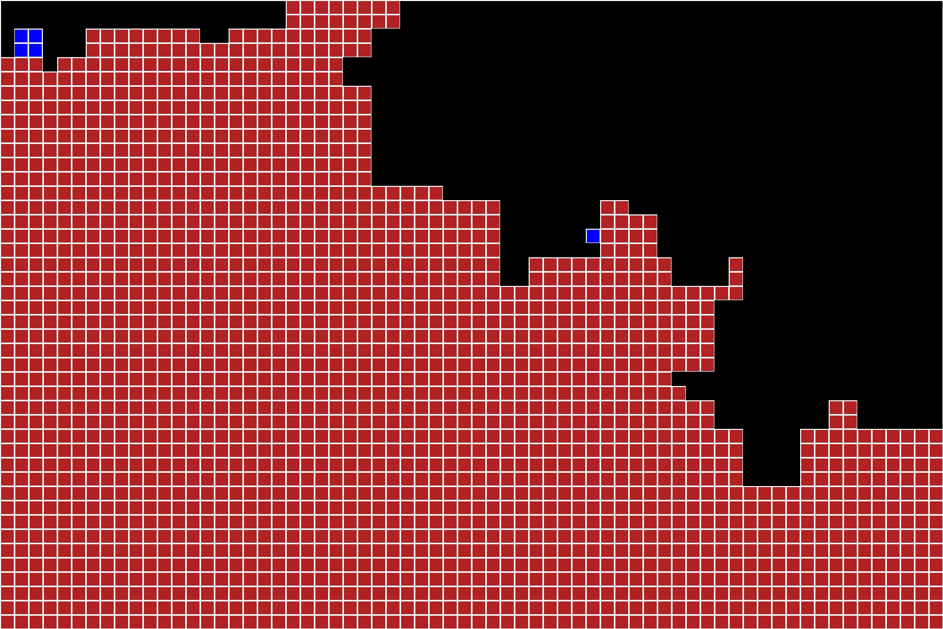
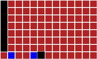
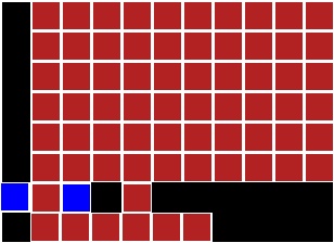
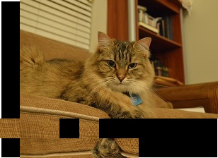
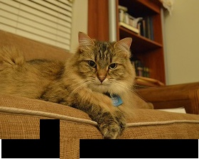
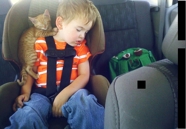
Interesting outputs from the solver:
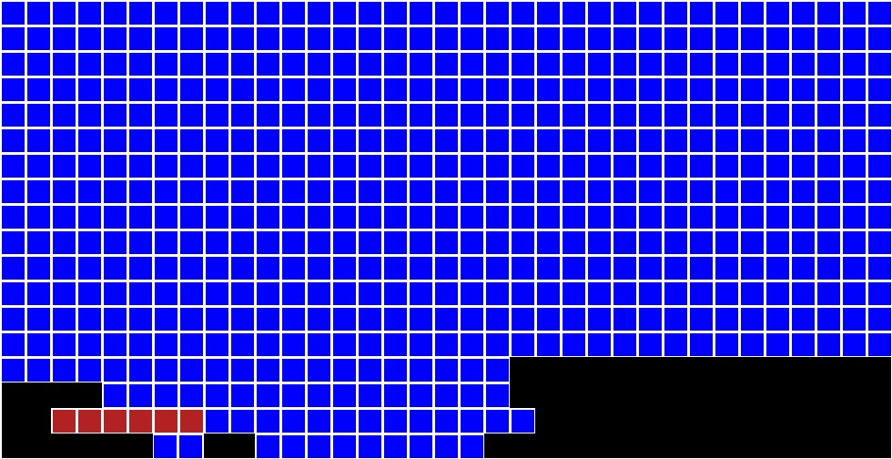
Note in the images below the black squares represent pieces that were not placed. These will eventually be filled in by the final solver one the feature to recalculate compatibilities is added.For this first image, I contrast the output from the original solver versus the Paikin Tal solver. Note that for type 1, both performed reasonably well although the Paikin Tal did have perfect accuracy for the placed pieces. For type 2 puzzles, Paikin Tal perform better with the exception that rather than placing the remaining pieces at the bottom of the board, it had a false positive on one end piece which caused the last few pieces to be incorrectly placed. This indicates the algorithm definitely has room for improvement.
| Solver | Type 1 Puzzle | Type 2 Puzzle |
|---|---|---|
Original "Naive" Implementation |
 |
 |
My Paikin & Tal Implementation |
 |
 |
One of the images from the McGill image dataset is buildings with one in the foreground and another in the background. This image is shown in Paikin and Tal's paper as a success case. Below is the image as a type 2 image from my solver. Note that the accuracy is quite high and only a couple of pieces are unplaced. The solver had markedly better performance on this image.
| McGill Image 20 |
|---|
 |
The current implementation of the Paikin and Tal algorithm also struggles with the Che Guevara image. Due to the nature of the Paikin and Tal algorithm requiring multiple pieces in type 1, I decreased the puzzle piece size from 50 to 25. It is also important to note that the original algorithm forced the board size into the right dimensions while Paikin and Tal's algorithm does not. In Paikin and Tal's solver, most of the face is correctly assembled; what appears to have happened is the lower left corner has shifted to the top right corner.
| Solver | Original Image | Type 1 Puzzle | Type 2 Puzzle |
|---|---|---|---|
Original "Naive" Implementation |
 |
 |
 |
My Paikin & Tal Implementation |
|
 |
|
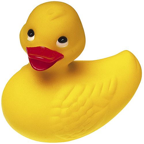
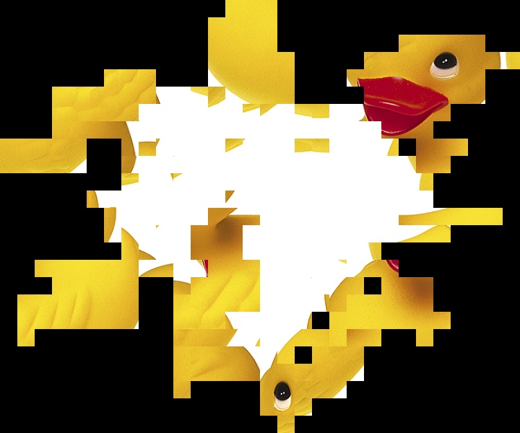
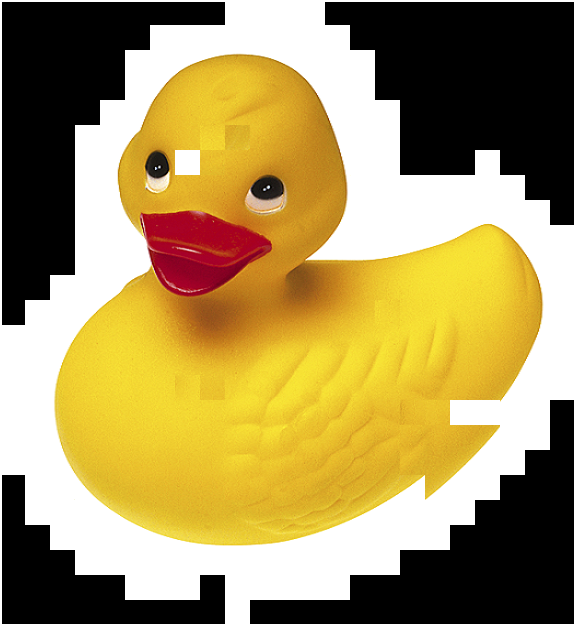
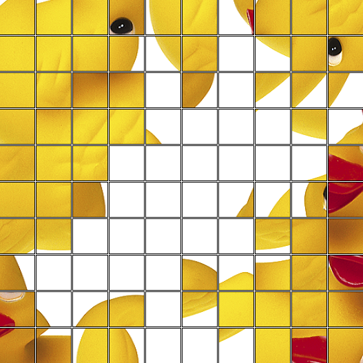
For the rubber duck, the Paikin and Tal solver overemphasized the white area. This is because the when two pieces are a direct match as the white space is, the mutual compatibility becomes irrelevant and all of them become their own best buddies. This caused the white space to cluster in the center, even on a type 1 image.
| Original Image | Paikin and Tal Type 1 Solver Solution |
|---|---|
 |
|
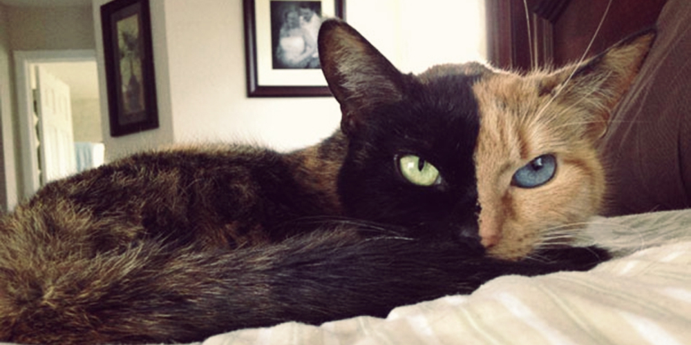
The last set of images I will show is the two face cat. My implementation of Paikin and Tal struggled with this image as it grew outside the bounds of the image.
| Original Image | Type 1 Result | Type 2 Result |
|---|---|---|
 |
 |
 |
Ideas meriting future consideration:
- Disallowing Multiple Best Buddies: The definition of a best buddy by Pomeranz et. al., Paikin & Tal, as well as others use greater than or equal to define best buddies (see for example equation 4 in Paikin and Tal's paper). However, this can give poor results in the case of images like Che Guevara and the duck, since in true solid areas, everything is everything else's best buddy.
- Use the Worst Case Mutual Compatibility: Paikin and Tal currently place a piece which has maximum compatibility with any open side/slot. However, this approach has room for improvement. For example, when placing a piece, it can have neighbors on up to four sides. Using only the best of the four to do the placement neglects all the bad information from the other sides. There should be some middle way in this approach.
- Resetting the Best Buddies Pool: If all the pieces in the best buddies pool are below a certain threshold, Paikin and Tal spawn a new board (assuming the algorithm is below the specified number of boards). If all the boards have been spawned, consider resetting the pool to get higher probability pieces.
- Focus on Documents Only: Dr. Pollett and I hypothesize that reconstructing documents may in many ways be a more difficult problem than reconstructing images. We may look into that as a possible thesis topic.
Summary of the Meeting on March 15, 2016:
In last week's meeting, Dr. Pollett and I decided that I would implement my own version of Paikin and Tal's jigsaw puzzle solver algorithm. In the first two weeks of the semester, I had written both a jigsaw puzzle generator and a very naive solver. While it may have been faster initially to reuse all or most of that code, I decided against doing so for the following reasons:- Use of the PIL Library: Python's PIL library does a great job for basic reading, writing, and resizing of images. However, it runs out of steam when one wants to do more advanced image editing analysis, much less computer vision. When considering alternatives, the two best options were either scikit-image or OpenCV. In the end, I went with OpenCV because it appeared to be an overall more powerful package.
- Individual Pixel-Based Image Analysis: My original naive implementation of both the solver and puzzle generator did most operations at the pixel level. While the pixel level will work, it is both more complicated to implemented and slower than doing vector or matrix based operations. What is more, it makes the code much more verbose. Had I known the power of NumPy originally, I would have used it. After doing some reading, I saw NumPy was a good fit here so I am now doing all of my mathematical calculations using NumPy.
- Lack of Focus on Runtime Performance: In my original implementation, I focused less on implementing for speed and more for adding features. For small puzzles, that approach worked well enough. However, I could see it was beginning to break down as I tried to solve larger images. In my new implementation, one of my goals is to make the tool run at speeds similar to what Taikin and Pal achieved.
- Lack of Multiple Puzzle Support: My original implementation never really conceived the idea that there may be pieces from multiple puzzles at once. When doing the implementation this time around, I made sure to include multiple puzzle support.
- Lack of Missing Piece Support: My previous implementation assumed that every piece in the puzzle would always be present. When doing the implementation this time around, I made sure that I ensured the code would be robust enough to handle missing puzzle pieces.
- OpenCV - Version 2
- NumPy
- OpenCV Image Importer: Working and Verified
- RBG to LAB Colorspace Conversion: Appears to be working.
- Puzzle Piece Generator: Appears to be working.
- Puzzle Piece Shuffler: Appears to be working.
- Puzzle Piece Reconstructor: Appears to be working.
- Asymmetric Distance Calculator: Appears to be working but needs more verification.
- Best Buddy Finder: Appears to be working but needs more verification.
Summary of the Meeting on March 8, 2016:
This is the last scheduled week of the literature review. I focused on two primary papers this week. They were:- Paikin & Tal - "Solving Multiple Jigsaw Puzzles with Missing Pieces - PDF" (2015)
- Son et. al. - "Solving Square Jigsaw Puzzles with Loop Constraints - PDF" (2014)
As outlined in my proposal for CS297, the next step after the literature review is to implement one puzzle solver technique. I had previously implemented a solver as described in my week #2 blog posting. My implementation for that solver was in retrospect rather poor as it did not incorporate many of the problem's latest techniques (and added complications). In this new implementation, I intend to try to duplicate the results of Paikan and Tal using their algorithm. This will eventually be used as a sort of "test bench" for new approaches and techniques.
Ideas meriting future consideration:
- Confident Placing of "Super Pieces" - Paikin and Tal focused on confidently placing blocks one by one in the puzzle. One of the important points in Son et. al.'s paper is the idea of building small loops. The benefit of this over Paikin's approach is that when I place pieces one at a time, I only can make a decision based off one border (generally). In contrast, when I place a 2 by 2 block of four pieces, I can make a decision of placement based off more borders. This may improve the placement accuracy.
Summary of the Meeting on March 1, 2016:
As mentioned in last week's blog post, this week I continued the literature review of existing work done on the jigsaw puzzle problem. I focused on two primary papers this week namely:- Sholomon et. al. - "A Genetic Algorithm-Based Solver for Very Large Jigsaw Puzzles - PDF" (2013)
- Paikin & Tal - "Solving Multiple Jigsaw Puzzles with Missing Pieces - PDF" (2015)
- Wu - "Using Probabilistic Graphical Models to Solve NPcomplete Puzzle Problems - PDF" (2015)
- Son et. al. - "Solving Square Jigsaw Puzzles with Loop Constraints - PDF" (2014)
Possible Area of Future Investigation: Sholomon et. al. mention in their paper (which is a really good read) the idea of puzzles with extra pieces that are not valid. This is essentially the idea of a "junk" piece that must be detected and discard. This may be a good topic for the thesis.
Summary of the Meeting on February 23, 2016:
As outlined in my CS297 proposal, the next three weeks will be devoted to performing a literature review of existing techniques and solutions to the jigsaw puzzle problem. I will be regularly uploading working copies of my presentation to GitHub. The list of papers I am looking at this week are:- Cho et. al. - "The Patch Transform and its Applications to Image Editing - PDF" (2008)
- Cho et. al. - "A Probabilistic Image Jigsaw Puzzle Solver - PDF" (2010)
- Pomeranz et. al. - "A fully automated greedy square jigsaw puzzle solver - PDF" (2011)
Update on Pickle Support:
As mentioned in last week's section "", one of the deficiencies of my existing implementation of the square jigsaw puzzle solver was the lack of support for Python's pickle page. This limitation has since been fixed and Pickle seems to be fully working.Comments on my Solver from Week #2:
As I read the different papers, I am compiling a list of comments on my existing solver:- Patch Size: In my original work, I was using patches of size 50px by 50px. In the literature, most patches are far smaller in size (e.g. 7px by 7px in Cho 2010).
- Red-Green-Blue (RGB): In Python's Pillow library, the default encoding of an image pixel is in RGB. In contrast, most of the literature uses LAB (Lightness and a/b color opponent dimensions.
Ideas meriting future consideration:
- Agglomerative Hierarchical Clustering - Nothing in the literate I had read so far describes the jigsaw puzzle problem in terms of hierarchical clustering, and I do not yet know why that is. When solving puzzles as I child, I would often start building many different unconnected groups at a time. Why not build many parts of the puzzle at once then try shuffling them around? This could be a type of hybrid top-down and bottom up approach.
- Focus Just on Maximizing Pairwise Accuracy - It seems to me an entire thesis topic would be how to maximize pairwise accuracy between pieces. As this predictor increases, the need for complex algorithms significantly decreases (to the point of being linear time if the pairwise accuracy is 1).
- Is patch reuse such a bad thing? - If I expect to get 100% accuracy, then I can appreciate why patch re-use would be an issue. However, if I get a better image be reusing a piece, maybe that is not su .
Summary of the Meeting on February 16, 2016:
This week I worked on a very basic bottom-up jigsaw puzzle solver; it is by no-means optimized. It was meant more as a learning vehicle to get experience with the problem. Below is the basic procedure:- Parse the original image into the specified grid size. Add all of the pieces to the "unexplored set."
- Select a single piece to serve as the seed of the puzzle. Currently I try to select a piece close to the center as a simplification of the problem. This piece is then added the the "frontier set."
- Compare all pieces in the unexplored set to all open sides (i.e. those where a new piece can be placed) of pieces in the frontier set. Select the piece and side with the minimum distance.
- Remove the piece with the minimum distance from the unexplored set and place it into the frontier set. Check whether minimum distance piece and its neighbors have no open sides. If they do not, remove them from the frontier set.
- Repeat the steps #3 and #4 until all pieces have been placed
The Danger of Image Borders:
Borders or solid areas around the edge of an image can be the most likely causes of an error. Take below this puzzle of Che Guevara (just a random image I selected; no political meaning intended).
The puzzle looks as though it should be very easy to solve. However, when it is run through the tool, it runs into a very obvious problem as shown below.
Notice how in the image, it put all of the white borders together because obviously there was no color difference between them. This caused the image to be split in two. This is the danger of relying only on micro-information
The Complication of Rotating Images:
Much of the previous work on the jigsaw puzzle problem did not allow piece rotation. I originally did not fully appreciate the great simplification that caused. In fact, not allowing rotation reduces the number of possible permutations by over 16 times. Takes this simple image of a large ship. When rotation is not allow, my tool is able to correctly identify solve the puzzle as shown below: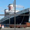
When rotation is enabled, the solution is very different.
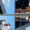
Notice how the two bottom pieces are placed side by side because of their similarity due to the brown ground. Again, this is the danger of relying solely on micro-information and not macro information.
Importance of the Distance Metric:
Depending on the distance metric, you may get very different puzzle solutions. The extent to which the solutions differed actually really surprised me. Below is the notation used to described each of the piece distance functions. Notation:- `p_i` : Piece `i`
- `w` : Width of the piece in pixels
- `c_(i,j)` : Color `j` for piece `p_i` in the (Red, Blue, Green) Spectrum
- `s_(i,k)` : `k^(th)` side (e.g. top, right, bottom, left) of piece `p_i`
- `d(p_n,p_m,s_(n,k))`: Distance between pieces `p_n` and `p_m` when `p_m` is placed on the `k^(th)` of `p_n`
Example #1: First Order where `d(p_n,p_m,s_(n,k)) = \sum_(w) \sum_j |c_(n,j)-c_(m,j)|`
Notice in this example, that the image has a large portion that is correct (the bottom half) and then the top half is all scrambled. This is explained in more detail later on.
Example #2: Ninth Order where `d(p_n,p_m,s_(n,k)) = \sum_(w) \sum_j |c_(n,j)-c_(m,j)|^9`
When the distance equation is increased to the ninth order, the image quality improves substantially overall. However, some of the pieces it got right before it now gets wrong (for example the lower right corner of the face).
Importance of a Single Misplaced Piece:
In example #1, you will notice that a single piece is highlighted in red. This piece was the 14 piece placed. This piece should have been placed near the bottom right corner. Until that point, only two pieces had been misplaced (highlighted in blue), and those two were simply transposed and could have been easily cleaned later. After piece 14 was placed, the quality of the solution dropped dramatically. Since the program does not currently fix a hard border around the board, the solution started growing vertically instead of horizontally.Remedy: If one piece can have such a deleterious effect, we need some way to detect such problematic moves and then to backtrack. The backtracking is the easy part; its the detection that is difficult.
Bigger is Not Necessarily Harder:
The difficulty of solving the puzzle seems much more to do with the texture of the image, than its size. Take two examples. In both, I place an the original image side by side with the puzzle solver's solution. Notice for the duck, the solver outputs a very poor image due to the substantial amount of solid colors and the border. The solution is so poor, one would be hard pressed to know it was a rubber duck. In contrast, take the "two-faced cat" which is exactly twice as large as the duck. While the solution is not ideal, most of the solution appears correct.| Original Image | Solver Solution |
|---|---|
 |
 |
 |
 |
Ideas meriting future consideration:
- Hybrid Bottom-Up and Top-Down - In a very tertiary view of the literature, I did not see any doing a hybrid bottom up and top-down approach. However, I think this is an idea that could work. It is also one of the best ways to get macro information about the picture. One simple way to do this secondary top-down search would be a local beam search.
- Using More than One Edge for Edge Distance: When building the puzzle, I currently treat each puzzle edge independently. However, that is often a poor strategy as I ignore the information from neighboring adjacent edges that may be useful. I also need to look if this is currently being done in other work.
- Fix Pickle Support - I noticed that when exporting a puzzle to Pickle that it was not importing properly. There have been some issues with Pillow in that regard. Not a showstopper, but worth fixing.
Summary of the Meeting on February 9, 2016:
The first deliverable as described in my proposal is a puzzle generator. This was originally scheduled to be a two week task. However, with some late nights and hard work, I was able to compress these activities into a single week. I have posted a description of the deliverable here.A few details:
- Language: Python (ver. 2.7.11)
- Puzzle Piece Board: Supports an optional board when exporting the solved/original puzzle.
- Puzzle Piece Rotation: Supports optional rotation of the puzzle pieces.
- Puzzle Piece Autosizing: Autosizes the puzzle and the pieces based off the specified grid size.
Ideas meriting future consideration:
- Bottom-Up versus Top Down: Humans solve puzzles in a bottom-up style by placing two pieces together. This makes sense because they already have macro information about the solution (e.g. the source image). In the absence of such macro-information, is it better for a computer to do a top-down approach?
- Unique versus Non-Unique Solutions: In some images (e.g. an all white picture), some pieces may be identical. We may want to consider as part of this research focus on only one of these two types of images or compare the two types.
- Solution Analysis Using the Fast Fourier Transform: It is anticipated that a source image may have a unique FFT signature. If that were the case, we may be able to use some version of the discrete fourier transform to quantify the quality of a puzzle solution.