Outline
- k-Means Clustering
- In-Class Exercise
- Community Mining
Introduction
- On Monday, we were talking about the analytics process model. This involves the steps: business process definition (of the business process we hope to analyze), data source identification and cleaning, ETL, data analysis and interpretation (where we actually try to use some analytical/machine learning technique on the data), interpretation of the results, and iteration.
- We talked about data source identification, cleaning, and ETL where we considered data pre-processing activities such as Denormalization, Sampling, Exploratory analysis, Missing Value Handling, and Outlier Detection and Handling.
- We then started talking about data analytics which we said comes in a variety of types: predictive, descriptive, survival, and social network analytics.
- We then focused on the first two of these.
- We said the goal of predictive analytics is to build a model that can be used to predict a target measure of interest. If the quantity is real valued then we call the model a regression model, if it is discrete (and usually finite) we call the model a classification model.
- We described how ordinary least square regression analysis can be done and the variants: Lasso regression and Ridge Regression.
- We showed how to do classification using logistic regression where we compose a linear model with the logistic function.
- We then considered descriptive analytics which tries to describe patterns of customer behavior and described hierarchical clustering as an example of this.
- We begin today by discussing a second way to do descriptive analytics using `k`-means clustering.
Norms
- As with hierarchical clustering, for `k`-means clustering our starting assumption will be that we have a collection of data points `vec{x_1}, ... vec{x_n}` in some space with a norm `|| cdot ||`.
- A norm is some mechanism to define the length of a vector which satisfies:
- `||vec{x} + vec{y}|| \leq ||vec{x}|| + ||vec{y}||` (triangle inequality)
- For any scalar `a` in the field our vectors are defined over (usually the reals), `||a\vec{x}|| = |a|||\vec{x}||`.
- If `||vec{x}|| = 0` then `\vec{x} = \vec{0}`.
- Some example norms are: `||vec{x}||_1 = \sum_i |x_i|` and `||vec{x}||_k = (\sum_i (|x_i|)^k)^{1/k}` for any fixed `k > 1`. When `k=2` this is the standard length of a vector you learn in calculus.
- Given a norm, we can define the distance between two points as `||vec{x} - vec{y}||`.
`k`-Means Clustering (McQueen 1967)
- `k`-means clustering is a non-hierarchical procedure that computes clusters `C_1`, ..., `C_k` according to the following steps:
- Select `k` points `vec{s}_1, ..., vec{s}_k` in our space as the initial cluster centroids (the seeds).
- Assign each data point `vec{x}_i` to the cluster `C_j` that has the closest centroid. This involves `k` comparisons to find the `j` such that `||vec{x_i} - \vec{s_j} ||` . Here
is where we are using a norm.
- For each cluster `C_j` created in this round, calculate a new centroid of its points: `\vec[s'}_j = 1/|C_j| sum_{vec{x} in C_j} vec{x}`.
- Check if `sum_{j=1}^k||vec{s'}_j - vec{s}_j|| \leq epsilon` where `epsilon` is some small real number that is our stopping condition.
- If yes, output our clusters, if no, set `vec{s}_j := vec{s'}_j` and recompute the above steps using the new seeds.
Choosing the Initial Seeds
- Forgy and Random Partition are two common techniques to assign the initial seeds.
- In Forgy, we choose `k` points at random from our data set as our initial seeds.
- In Random Partition, we cycle through the data set, assigning each data point `vec{x}_i` at random to some cluster `C_j`. Then we use the centroids of this initial set of clusters as our starting seeds.
Choosing `k` in `k`-Means - the Elbow Method
- One way to measure how good at set of clusters is, is to compute the Within-Cluster-Sum of Squared Errors (WSS) `\sum_{j=1}^k \sum_{vec{x} in C_j} ||vec{x} - s_j||^2`.
- So one technique to determine a good choice of `k` is to plot (WSS) versus `k` and look for a value of `k` for which this stops decreasing by much. This is called the Elbow method.
In-Class Exercise
- Randomly generate 20 points in the plane by rolling two six sided dice (one for the `x` value, one for the `y` value). For the first, 5 rolls use the pairs that you get directly, for the next five add 5 to each coordinate, for the five after that 10 to each coordinate, and for the last five 15 to each coordinate.
- For `k = 3,4,5`.
- Create initial seeds using forgy. Then compute the `k` means clusters according to our algorithm.
- Do you observe an elbow in a plot of the WSS?
- Please post your work and answer to the May 8 In-Class Exercise Thread.
Social Network Analytics
- Social Network Analytics is analysis of data sets coming from a social networking site such as Facebook, X, LinkedIn, etc.
- For us a social network consists of nodes and edges, each typically labelled with multiple attributes (how such a network is different than just a graph).
- For example, nodes could be viewed as a customer, household, patient, doctor, author, etc each with their own attributes like name, id, income, etc.
- An edge could represent a relationship such as a friend, a call, a contact, a disease transmission. Edges might have real valued weight representing for example, strength of friend contact, frequency of calls between two people, etc. The latter might be used for predicting how like a company likely Skype is to lose a customer (churn).
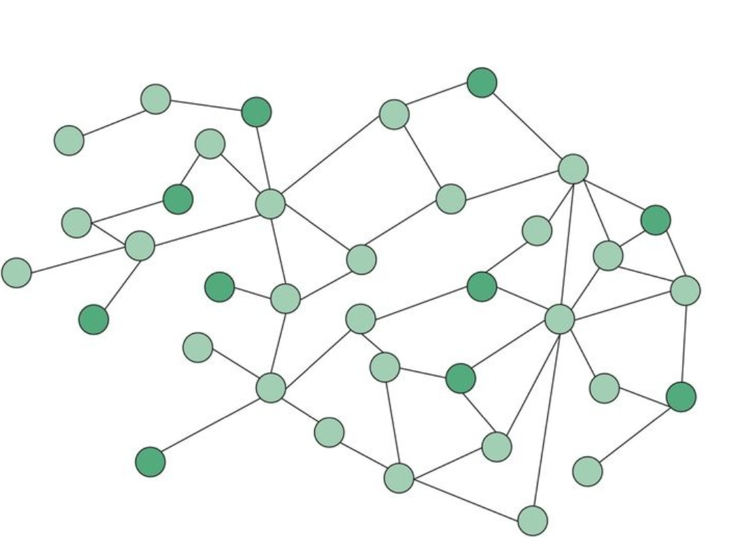
- Social networks can be represented in a diagram called a sociogram. The image above is a sociogram where the color of nodes correspond to churner/non-churner status.
- Such graphs are helpful for smaller networks, for larger networks typically weighted adjacency matrices are used.
Social Network Metrics
- A social network is often characterized using various centrality metrics such as:
- Geodesic - Shortest path between two nodes in the network.
- Degree - Number of connections of a node.
- Closeness - The average distance of a node to all nodes in the network.
- Betweenness - A count of the number of times a node or edge lies on the shortest path between any two nodes in the network.
- Graph theoretic center - The node with the smallest maximum distance to all other nodes.
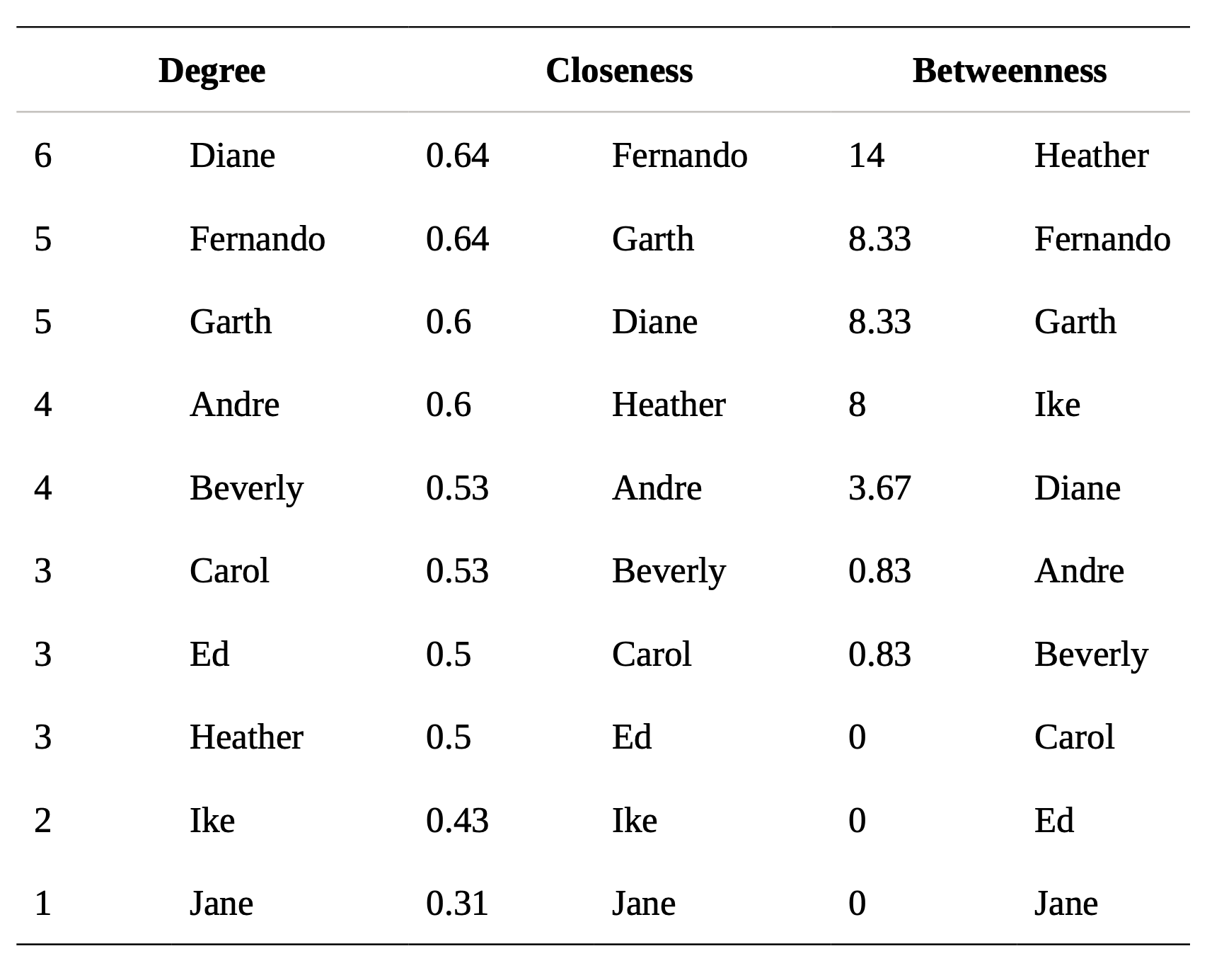
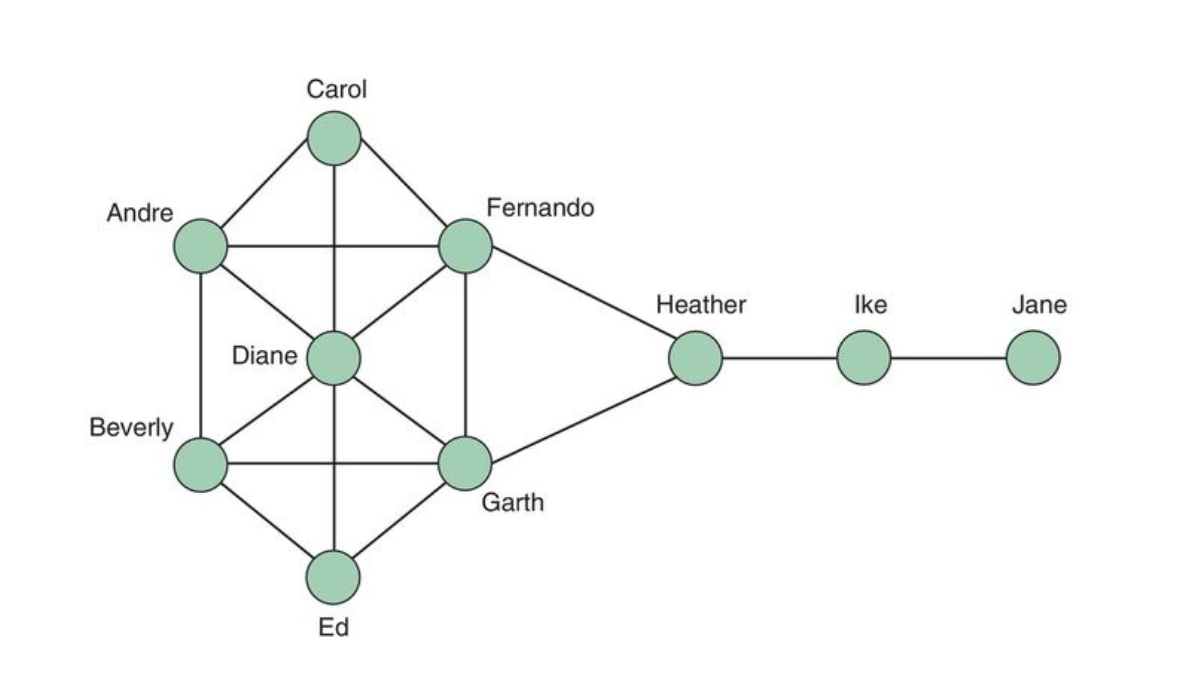
- The table on the right shows the values of some of these metrics for the graph on the left.
Community Mining
- In the graph of the previous slide, Heather had the highest betweenness.
- She sits between the two communities {ike, Jane}, and everyone else.
- This hints that betweenness might be useful for community mining.
- One popular mining technique called the Girvan-Newman algorithm is as follows:
- Calculate the betweenness of all edges in the network
- Remove the edge with the highest betweenness.
- Recalculate the between of all edges in the network
- Repeat (2) and (3) until no edges remain.
- As the algorithm runs we essentially get a dendogram of the communities of different scale where nodes all whole graphs, we have an edge from graph B to graph A if B is a subgraph of A with fewer nodes and A and B differ in structure by they removal of one edge. I.e., the first edge removal that causes the graph to become disconnected
would be the first pair of communities and so on.


