Introduction

For our final topic this semester, we are going to look at analytics.
We have already looked at how to extract, transform, and load data into a data warehouse.
The point in putting data into a data warehouse was to allow us to analyze data to inform our business or organizational decision.
So by analytics, we mean techniques to actual do this.
Analytics often also goes under the name of data science, data mining, knowledge discovery, and predictive or descriptive modeling.
To start we begin by looking at the overall analytics process...

Analytics Process Model

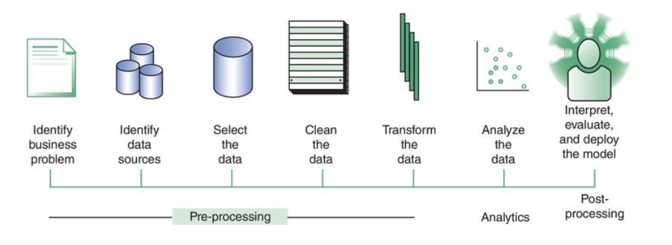
The above figure shows the analytics process model.
Let's briefly look at these steps:
- Business Process Definition - Some example business processes include: customer segmentation of a mortgage portfolio; retention modeling for a postpaid telecom subscription; or fraud detection for credit cards. As part of the definition process, a data scientist and a business expert need to agree on key concepts, such as how to define a customer, transaction, churn, fraud, etc.
- Source data Identification, Data Selection, Data Cleaning, Transformation - these steps are typically what is involved in getting the data into a data warehouse.
- Data Analysis - here an analytical model is estimated on the pre-processed and transformed data. Depending upon the business problem, a particular analytical technique will be selected and implemented by the data scientist.
- Interpretation - this is done by a business expert. Trivial patterns might be used such as spaghetti and spaghetti sauce are often purchased together to validate the analytics model. Once the model is validated, the goal of this step is to find the unknown but interesting and actionable patterns (nuggets) that can provide new insights into your data. Once the analytical model has been appropriately validated and approved, we then want to make sure deploy it as a user-friendly application to allows us to extract useful nuggets in an ongoing basis.
- Iterate - The whole model above is iterative. At each step in the model, we might decide we need to go back and improve what we did at some earlier step to make sure we get the analytics application we want in the last step.
Some key actors in who need to be involved in the above process model are: (a) The DBA for data warehouse. (b) The business expert for the business process being analyzed. For example, maybe credit portfolio manager for the mortgage portfolio process. (c) Legal experts who are aware of laws which govern what data can be used for analytics due to privacy, discrimination, and other issues, (d) software tool vendors for the analytics modeling software, (e) the data scientist doing the actual analytics.

Applications

Let's look at some ways that analytics can be used to optimize business decisions:
- Risk Analytics - the use of analytics to measure, predict, and mitigate risk. For example, financial institutions use analytics to build credit scoring models to gauge the creditworthiness of their customers on all their credit products. The government uses fraud analytics to predict tax evasion, VAT fraud, or for anti-money laundering tasks.
- Market Analytics - the use of analytics for marketing decisions. Some of example of techniques in this area are: churn prediction (how many customers likely to leave a service in a given time period), response modeling (try to determine which customers are most likely to respond to what kind of marketing campaign), and customer segmentation (cluster transactions into homogeneous groups of customers for marketing purposed)
- Recommender Systems - these aim to provide well-targeted recommendations to a user. For example, Yelp might recommend a restaurant to a user based on past reviews visited or uploaded by that user.
- Text Analytics - this aims at analyzing textual data such as reports, emails, text messages, tweets, web documents, blogs, reviews, financial statements, etc. For example, Facebook and Twitter are continuously performing using social media analytics to study both their content and sentiment.

Data Preprocessing

The point of data preprocessing is to make sure that our analytics system gets good quality data in, so that good quality decisions can be made from it. I.e., we want to avoid a garbage in garbage out situation (GIGO).
Some important data preprocessing activities are:
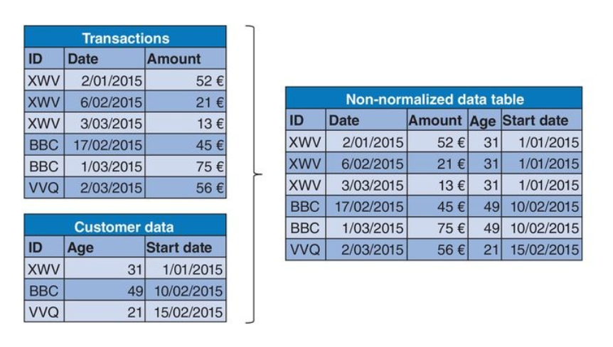
- Denormalization - for analytics we usually assume the data comes in as a single big table, i.e., the opposite of what we are taught to do in database design classes. The process of going from our data we need for analysis being distributed across many tables to being consolidated, aggregated, and merged into one or at most a small of tables (see figure above) is called denormalization.
- Sampling is the use of a subset of the whole dataset (say, some number of past transactions) to build an analytic model. The key here is to determine a subset which will be most useful for making future predictions. So one might have a tradeoff between lots of data (and hence a more robust analytical model) and recent data (which may be more representative).
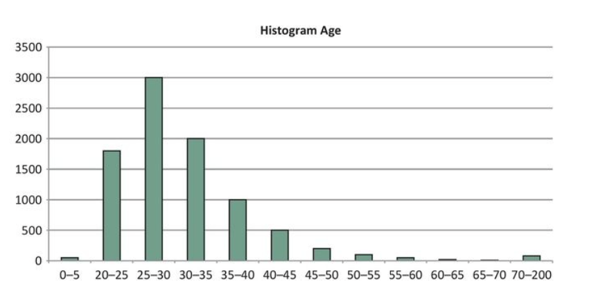
- Exploratory analysis involves making charts, graphs, etc, to get to know your data in an "informal way". A chart like the histogram above for age distributions is an example. These initial insights into the data can be adopted throughout the analytical modeling stage.
- Missing Value Handling - missing values might occur for a variety of reasons: the information is non-applicable, non-disclosed, errors during merging (caused by typos). These missing values may indicate patterns. For example, a missing value for income, may indicate unemployment. To handle missing value, one often either: (a) removes the data item, or (b) replaces the value with an average or median.
- Outlier Detection and Handling Outliers are extreme observations that are very dissimilar to the rest of the population. For example, someone whose age is 300, or a person such as a CEO whose salary is much larger than all of the employees. Graphical tool like histograms, box plots, and scatter plots can also a data scientist to see data points that are likely to be outliers. Removing outliers can be useful as some analytics techniques such as linear/logistic are sensitive to them. Other techniques such as decision trees are not. Often after using such a graphical tool, a data scientist can choose caps on the values to be included into a data set to remove outliers.

Types of Analytics

We now look at some different techniques used to carry out analytics.
The aim being to extract valid and useful business patterns or mathematical decision models from a pre-processed dataset.
We are going to look at: predictive analytics, descriptive analytics
Two other kinds of analytics are: survival analysis, and social network analytics.

Predictive Analytics

The goal of predictive analytics is to build a model that can be used to predict a target measure of interest.
It can be dinstinguished into two subtypes of analytics:
- Regression where the target value is continuous, for example, sales, stock prices, etc.
- Classification where the target value is one of a fixed list of categories. For example, a binary classifier might predict whether or not something happens such as defaulting on a loan.

Regression

One popular approach to regression is to use some kind of curve, surface, or hypersuface fitting.
For example, in linear regression, we try to find the "best hyperplane", `y = f(vec{x}) = beta_0 + beta_1 \cdot x_1 + cdots + beta_n \cdot x_n`, corresponding to a set of data points {`(vec{x}_0, y_0)`, ..., `(vec{x_k, y_k})`}.
By best hyperplane, we mean one that minimizes some loss function over the dataset. A possible loss function might be something like least square errors: `sum_{i=0}^k (|y_i - (beta_0 +vec{beta}^T\vec{x_i})|)^2`.
Other loss functions might change the square above to some different power or add so called regularization terms to avoid sensitivity to outliers. For example, `sum_{i=0}^k (|y_i - (beta_0 +vec{beta}^T\vec{x})|)` corresponds to a Manhatten distance loss function.
Finding the minimum of a loss function typically involves computing a gradient of the loss functions and then use some kind of steepest descent method to find where the gradient is 0 (i.e., in this case a minimum).
Once, we have a found a `vec{beta}` which minimizes the loss on the data, we can then start making predictions. If you give me some new point `vec{w}`, I can find the corresponding `y` prediction by computing `f(vec{w})`.

Classification

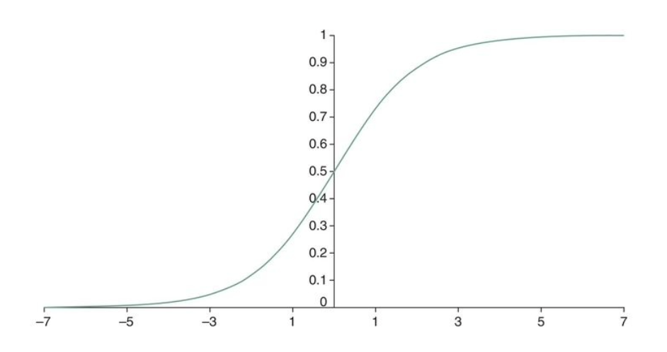
By composing our linear model, with the logistic function, `f(z) = 1/(1+e^{-z})` (see graph above), to get a function `1/(1+e^(-(beta_0 +vec{beta}^T\vec{x})))` which can be used for classification.
Curve fitting for this kind of function is called logistic regression.
Another approach to classification is to use decision trees.
Once we have a classification model, we often want to measure how good it is one some kind of test data set.
This is a whole area in itself, but some example measure that can be used are (T=true, F=False P=positive, N=negative):
- Classification accuracy = (TP + TN)/(TP + FP + FN + TN),
- Classification error = (FP + FN)/(TP + FP + FN + TN) ,
- Sensitivity = Recall = Hit rate = TP/(TP + FN),
- Specificity = TN/(FP + TN)

Descriptive Analytics

Descriptive Analytics tries to describe patterns of customer behavior.
Some techniques in this area are: association rules and variations on clustering.
Association rules are rules aimed at detecting frequently occurring associations between items. For example, one might try to determine sets of items which are frequently purchased together such as: Baby food, beer, diapers, milk.
One algorithm to do this is the A Priori algorithm.
In clustering, we want to split a set of observations into clusters so the homogeneity within a cluster is maximized (cohesive), and the heterogeneity between clusters is maximized (separated).
The two most common approaches to clustering are hierarchical clustering and k-means clustering. We will only look at the former, but the book describes both.

Hierachical Clustering

In this kind of clustering we assume we have some kind of distance function between items in out data set. For example, if we were clustering cities into larger geographic regions, we might use Euclidean distance.
Using this distance function, we then build a tree out of our data items in either a top down or bottom up fashion. We will only consider the bottom up fashion (agglomerative).
We start off with a forest of single item clusters.
We then take the two clusters in this forest which are closest to each other, we combine them to make a tree whose parent node has all of the elements of the child clusters.
We repeat this process on the resulting forest of clusters until our forest consists of a single tree.
Although, the distance function `d` might be between items in our dataset, one can extend it to a distance function between clusters in one of various ways. For example, `d(c_1, c_2)` could be the average distance between elements in the two clusters or the min or max distance between any two elements in the two clusters.
If we want some fixed number `k` of clusters rather than the whole tree, we stop the above process when we have only `k` clusters left.

Analytics

Outline

Introduction

Analytics Process Model

Applications

Data Preprocessing

Types of Analytics

Predictive Analytics

Regression

Classification

Descriptive Analytics

Hierachical Clustering

In-Class Exercise