Outline
- Unfolding Computation Graphs
- In-Class Exercise
- Designing RNNs
- Gradient Descent for RNNs
- Bidirectional RNNs
- Encoder-Decoder Sequence-to-Sequence Architecture
Introduction
- Last day we began talking about neural networks that could handle sequential data.
- We said recurrent neural networks were one way to do this.
- We imagine RNNs as operating on data with time indexes. So `\vec{x}^{(t)}` would be the the `t` item received to
the neural net.
- We imagine `t` running from 1 to some number `tau`.
- The value `t` might represent a time or it could represent a position. For the example, the `t`th word in a document.
Unfolding Computation Graphs
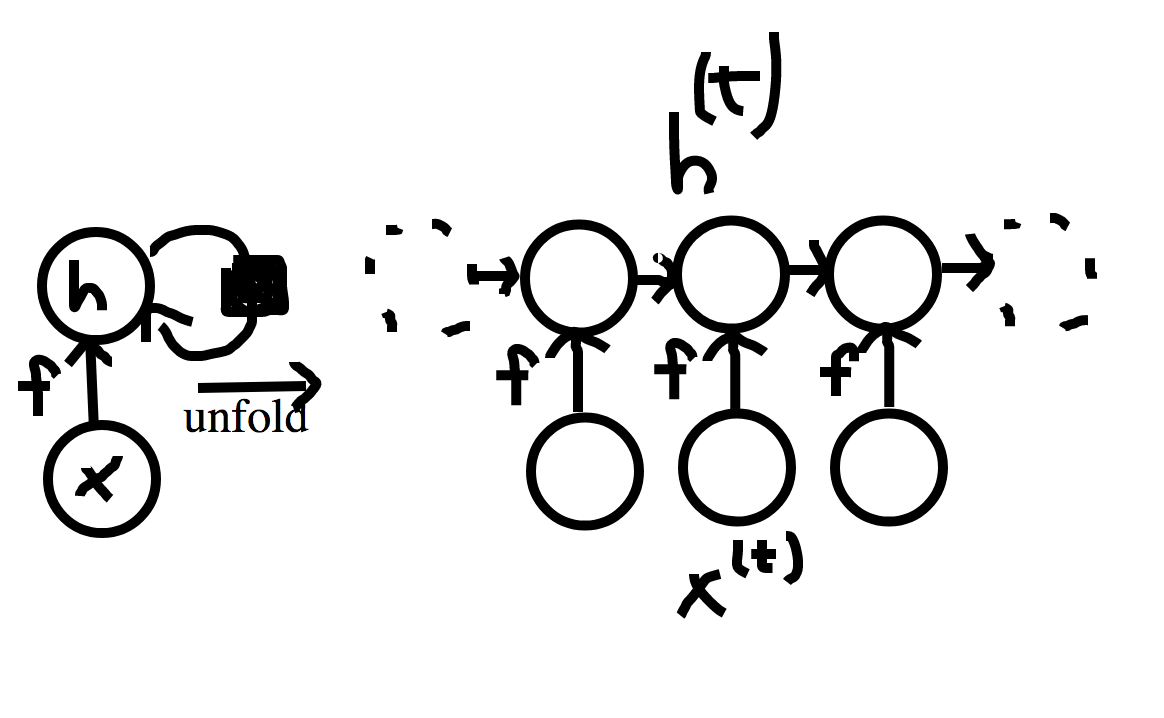
- Suppose we have a hidden layer in our neural net that computes some recurrent function.
- We write this as:
`vec{h}^{(t)} = f(vec{h}^{(t-1)}, vec{x}^{(t)}; theta)`
- Thus, the output of the hidden layer at time `t` is a function of the value of the hidden layer at time `t-1`, the data received at time `t`, and the network weights.
- Notice the network weights don't change with time.
- Two common ways to draw the computation graph for this layer are shown above.
- The left hand side shows just the state at a given time, with the black box on the edge from `\vec{h}` to
`vec{h}` indicating that this node receives a previous value with a time delay of 1.
- The right hand side show the graph unfolded and how the previous values of `vec{h}` get fed into next.
- We will sometimes write `vec{h}^{(t)} = g^{(t)}(vec{x}^{(t)}, vec{x}^{(t-1)}, ..., vec{x}^{(1)})` for `f(vec{h}^{(t-1)}, vec{x}^{(t)}; theta)`.
- Here `g^{(t)}` is the function that operates on the complete unfolding.
Advantages of RNNs
- Regardless of the sequence length, the model learned always has the same input size. This is because it is specified in terms of the
transition from one state to another, rather than in terms of a variable-length history of states.
- The same transition function `f` is used with the same parameters at every step. Hence, we are learning a single model `f` that operates on
all time steps, and all sequence lengths, rather than needing to learn a separate model `g^{(t)}` for each number of time steps.
In-Class Exercise
- Let `x^{(1)}, ... x^{(\tau)}` be a binary sequence. I.e., each `x^{(i)} in \{0, 1\}`.
- Suppose we want `h^{(vec{t})}` to output the number of 1's in `x^{(1)}, ..., x^{(t)}` mod 8. using an RNN.
- How many neurons would we need for `f`? How many inputs should each neuron get?
- Completely describe each neuron needed to compute `f`.
- Please post your solution to the Nov 10 In-Class Exercise Thread.
Designing Recurrent Neural Nets
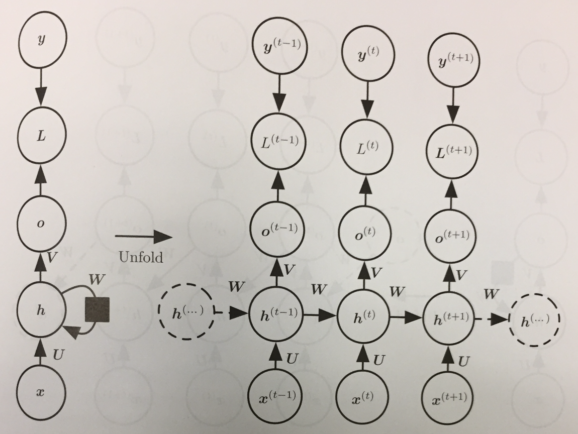
- Using our two computation graph models for RNNs we can express three common design patterns for RNNs:
- An RNN that produces an output at each time step and has recurrent connections between hidden units:
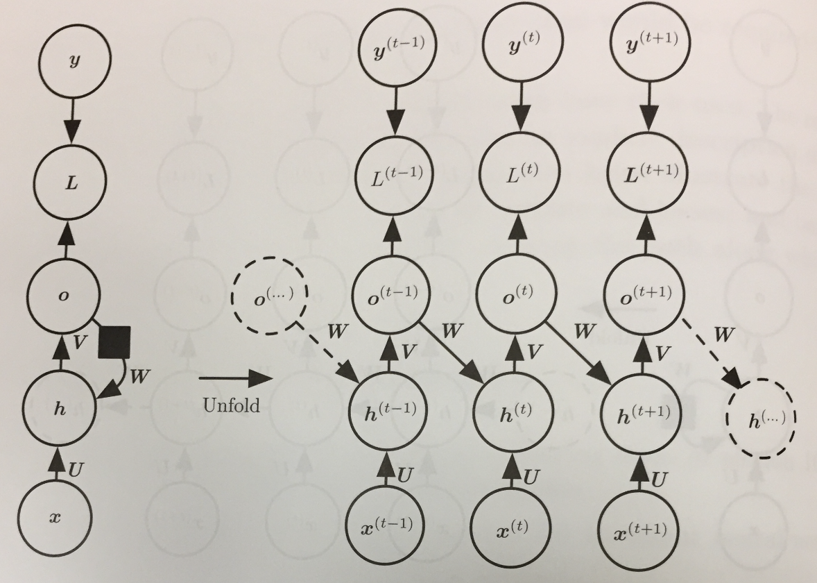
- An RNN that produces an output at each time step and has recurrent connections only from the outputs at one step to the hidden units
at the next:
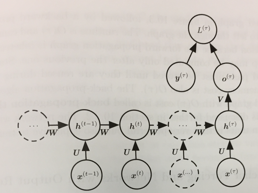
- An RNN with recurrent connections between hidden units, that reads the entire sequence, and then produces a single output:
Converting Graphs to Forward Propagation Equations
- Siegelmann and Sontag (1991), Siegelmann (1995), and Siegelmann and Sontag (1995) show how to use the first architecture of the previous slide to
implement arbitrary Turing Machines. Hence, any computable function can be implemented using such an architecture.
- Let's focus for the moment on just understanding the recurrence functions the first graph is saying to compute.
- Forward propagation needs to assume some initial state for the hidden layer: `vec{h}^{(0)}`.
- Given this, the update equations used to compute an output vector `hat{y}^{(t)}` are:
\begin{eqnarray*}
\vec{a}^{(t)} & = & \vec{b} + W \vec{h}^{(t-1)} + U \vec{x}^{(t)}\\
\vec{h}^{(t)} & = & \tanh(\vec{a}^{(t)})\\
\vec{o}^{(t)} & = & \vec{c} + V\vec{h}^{(t)}\\
\hat{y}^{(t)} & = & \mbox{softmax}(\vec{o}^{(t)})
\end{eqnarray*}
- The top of the diagram is for training. If `L^{(t)}` is the negative log-likelihood of `y^{(t)}` given `vec{x}^{(1)}, ..., vec{x}^{(t)}`, then
\begin{eqnarray*}
L(\{\vec{x}^{(1)}, ..., \vec{x}^{(\tau)}\}| \{\vec{y}^{(1)}, ..., \vec{y}^{(\tau)}\}) & = & \sum_t L^{(t)}\\
& =& - \sum_t \log p_{\mbox{model}}(y^{(t)} | \{\vec{x}^{(1)}, ..., \vec{x}^{(t)}\})
\end{eqnarray*}
- Here `p_{\mbox{model}}(y^{(t)} | \{\vec{x}^{(1)}, ..., \vec{x}^{(t)}\})` is the `y^{(t)}` entry from the output vector of the model `hat{y}^{(t)}`.
Backpropagation Through Time
- To compute the gradient of the just presented network involves performing a forward pass moving left to right through the unrolled computation graph.
- This is then followed by a backward propagation pass moving right to left through the graph.
- Together this gives a runtime of `O(\tau)` and a memory cost of `O(\tau)`.
- This process is called back-propagation through time (BPTT) and can be very expensive because it can't be easily parallelized as the forward graph is sequential in nature and we need
to remember each value for the backward pass.
Teacher Forcing, Networks with Output Recurrence
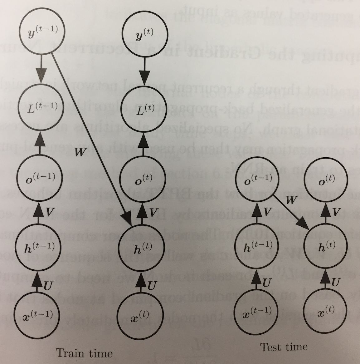
- If we look back to the second of the three common RNN design patterns, we see that it does not involve recurrences from hidden layers to hidden layers.
- Instead, the outputs lead back into the model.
- This allows for teacher forcing training which avoids having to do the more costly BPTT.
- Rather than feeding the model's own output back into itself during training, we can use just the sequence `\vec{x}^{(1)}, ..., \vec{x}^{(t)}` so far, `vec y^{(t)}` and `vec y^{(t-1)}`,
where we can think of `vec y^{(t-1)}` as a teacher forcing what the previous answer should be.
- The drawback of teacher forcing is that in an open loop, test time situation, where the networks outputs are fed back as inputs, it might not perform as well as our first model.
- The book gives some suggestions of how to mitigate this problem.
Gradient Descent for RNNs
- To perform gradient descent through an RNN one applies generalized back-propogation on the unrolled computation graph.
- To gain some intuition on how BPTT behaves, let's consider the equations `\vec{o}^{(t)} = \vec{c} + V\vec{h}^{(t)}`, `\hat{y}^{(t)} = \mbox{softmax}(\vec{o}^{(t)})`, and our equation:
`L(\{\vec{x}^{(1)}, ..., \vec{x}^{(\tau)}\}| \{\vec{y}^{(1)}, ..., \vec{y}^{(\tau)}\}) = \sum_t L^{(t)}.`
- For each node `N` we need to compute the gradient `grad_N L` recursively based on the nodes that followed it in the graph.
- We note `(del L)/(del L^{(t)}) = 1`.
- We assume that the loss is is the negative log-likelihood of the true target `y^{(t)}` given the input so far. I.e., `L^{(t)}` is `- log (hat{y}_{y^{(t)}}^{(t)})`.
- Then
`(grad_{\vec{o}^{(t)}} L)_i = (del L)/(del \vec{o}_i^{(t)}} = (del L)/(del L^{(t)}) (del L^{(t)})/(del \vec{o}_i^{(t)}} = 1 cdot( - (del \hat{y}^{(t)})/(del \vec{o}_i^{(t)}})/(hat{y}^{(t)}) = hat{y}^{(t)} - vec{1}_{i, y^{(t)}}`.
- We are using here that softmax enjoys similar properties to the logistic function `sigma(x)` which satisfies `sigma(x)' = sigma(x)(1 - sigma(x))`.
- The only descendent of `vec{h}^{(\tau)}` is `o^{(tau)}` so its derivative is `grad_{vec{h}^{(\tau)}} L = V^{top}grad_{vec{o}^{(\tau)}}L`.
- To compute the gradients of `vec{h}^{(t)}` for `t < \tau` we note `vec{h}^{(t)}` is a descendent of both `vec{o}^{(t)}` and `vec{h}^{(t+1)}`, so:
`grad_{vec{h}^{(t)}} L = ((del vec{h}^{(t+1)})/(del vec{h}^{(t)}))^{top} grad_{vec{h}^{(t+1)}} L + ((del vec{o}^{(t)})/(del vec{h}^{(t)}))^{top} grad_{vec{o}^{(t)}} L`
`= W^{top}(grad_{vec{h}^{(t+1)}} L) diag(1 - (vec{h}^{(t+1)})^2) + V^{top}grad_{vec{o}^{(t)}} L`
Here `diag(x)` is the diagonal matrix with `x` repeated on the diagonal.
- The book shows how to continue to iterate back to compute the gradients for each of the equations in our first design pattern model.
Bidirectional RNNs
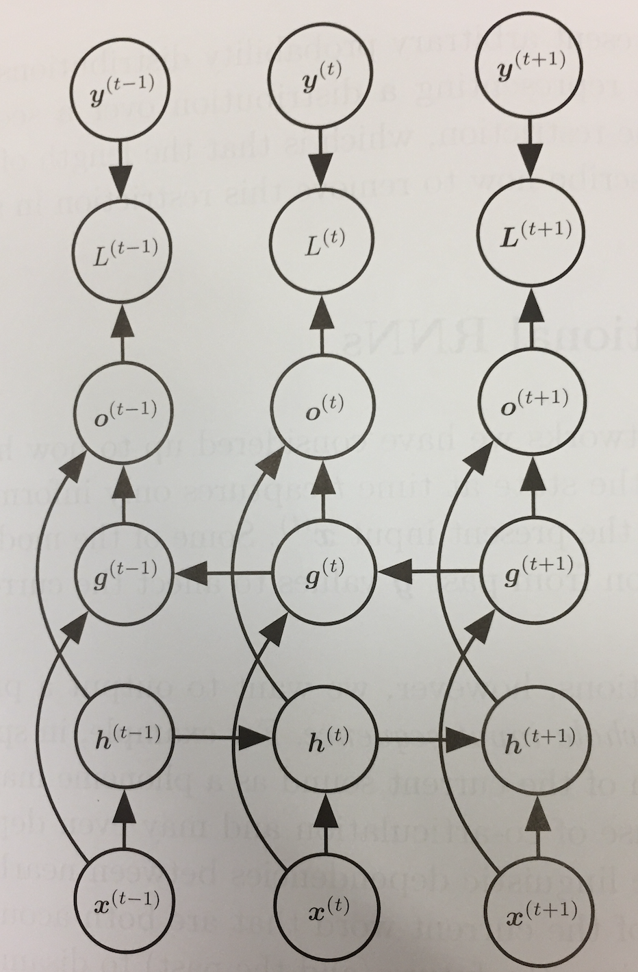
- Consider the problem of speech recognition. The correct interpretation of the current sound at time `t` might depend not only on the sounds earlier than `t` but also on sounds that appear after `t`.
- This is also true of handwriting recognition and other sequence-to-sequence learning tasks.
- Bidirectional RNNs were invented to solve this problem.
- They combine an RNN that moves forward through the sequence with another that moves backward through the sequence.
- In our above computational graph diagram, `vec{h}^{(t)}` is the state of the forward RNN, and `vec{g}^{(t)}` is the state of the backward RNN.
- The output units `vec{o}^{(t)}` depend on both of these and so will depend on both past and future values of the sequence.
- It will be most sensitive to the input values around time `t` without needing to specify a fixed window size.
Encoder-Decoder Sequence-to-Sequence Architectures
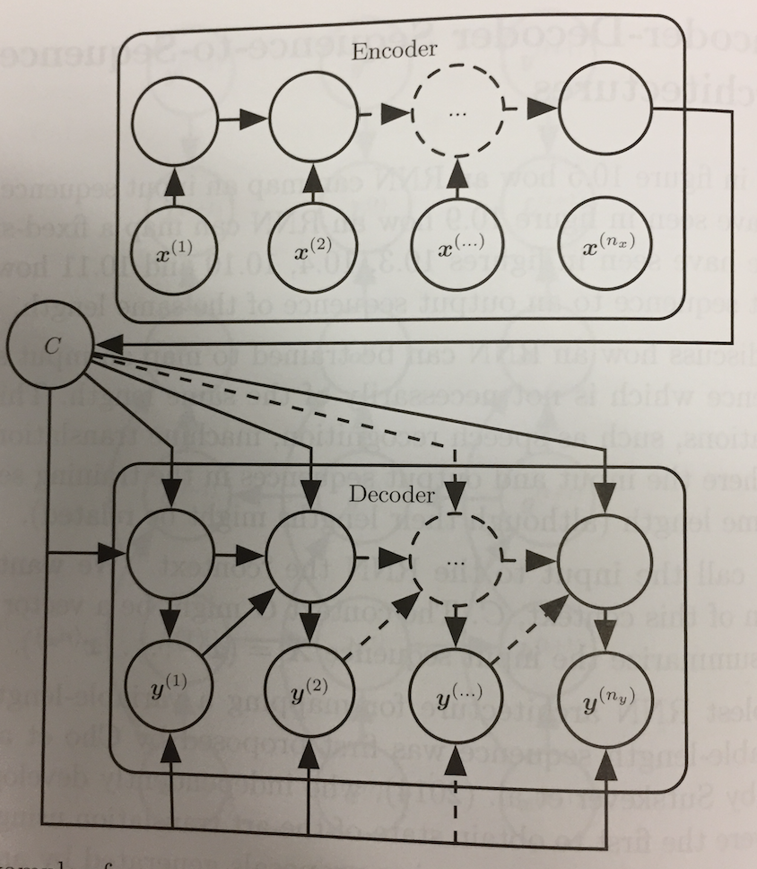
- So far our RNNs produce a sequence either of the same length as the input sequence (Design patterns 1 and 2) or produce a sequence of some fixed length (Design pattern 3).
- If you have ever looked at a Canadian cereal box, you know the same statement in one language (English) might be of a different length in another language (French).
- Cho et al (2014) and Sutskever et al (2014) independently proposed an encoder-decoder (aka sequence-to-sequence) architecture
to make it possible to have source and output sequences of different length.
- The model has two parts:
- An encoder RNN processes the input sequence `vec{X} = (vec{x}^{(1)}, ..., vec{x}^{(n_x)})` and emits a fixed length context `C` as a function of its final hidden state.
- A decoder RNN takes as one of its inputs this vector to generate an output sequence `vec{Y}= (vec{y}^{(1)}, ..., vec{y}^{(n_y)})`
- Here `n_x` and `n_y` can vary.
- Notice each node in the image of the decoder above gets `C` together with the previous value `vec{y}^{(t)}`. We can imagine having a code for the end of sequence to say when to stop generating.


