Introduction

On Monday, we began talking about SVMs (Support Vector Machines) (Cortes Vapnik 1995).
These are different than perceptrons in three main ways:
1. An SVM is computed by taking the inputs, applying a vector-valued function `vec{f}:RR^n -> RR^m` and then sending the result to a perceptron gate. The hope is that `vec{f}` maps the underlying classification problem into a space where it is separable. (We showed if you allowed `m` to be big enough this is always possible.)
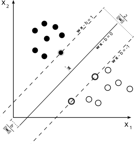
2. The computation of the weights for the perceptron portion of the SVM is done by computing a maximal margin separator of the classes being separated. Doing this will likely mean the model will generalize to new data better than if the weights were determined by the perceptron or Winnow rules. This is because in the latter cases, the separating hyperplane might be closer to one of the two classes than the other.
3. SVM training often makes use of soft margin techniques (haven't talked about yet) to handle the case where the data received by the perceptron is not separable.
We said that the usual way to find the separator for an SVM is by solving a quadratic program (a system of quadratic inequalities).
The SVM one gets is a threshold of terms like `vec{f}(vec{x}) cdot f(vec{x_j})`. The kernel trick involves avoiding the computation of `vec{f}` by directly computing a simpler function `k(vec{x}, vec{x_j})` for some kernel function `k`. Here `k` usually involves computing a dot-product `vec{x} cdot vec{x_j}` in the original space followed by a simple function of the reals.
We now continue our discussion of SVMs.

Computing Separators

For this discussion, `y_i` is 1 for a positive example and `-1` otherwise. Coordinates of `vec x_j, vec x_k` can be positive, 0, or negative reals.
Let's consider the problem of computing the maximal separator assuming we didn't do any mapping `vec{f}`.
The standard way to do this reduces the problem to solving a quadratic program: Maximize
`mbox(argmax)_(vec alpha) (sum_j alpha_j - 1/2 sum alpha_j alpha_k y_j y_k (vec x_j cdot vec x_k))`
subject to `alpha_j ge 0` and `sum_j alpha_jy_j = 0`.
Here the weights of the output SVM are related to the `alpha_j`'s above via the equation `vec w = sum_j alpha_j vec x_j`.
A classifier can be built out of `vec alpha` directly using the equation:
`h(vec x) = sign(sum_j alpha_j y_j(vec x cdot vec x_j) - b)`
which also only uses the data in a dot product.
An important property of the `alpha_j`'s is that they are `0` usually except the support vectors -- the closest vectors to the separator (typically in each dimension).
If we want to do a mapping `vec{f}` before computing the separator, the process is almost identical, except now the classifier becomes: `h(vec x) = sign(sum_j alpha_j y_j(vec{f}(vec x) cdot vec{f}(vec x_j)) - b)`
For some `vec{f}` we can replace the `(vec{f}(vec x) cdot vec{f}(vec x_j))` in classifier and `(vec{f}(vec x_j) cdot vec{f}(vec x_k))` in the quadratic program with a simpler to compute kernel function `k(vec{x}, vec{x}_j)` or `k(vec{x_j}, vec{x}_k)`.
A result known as Mercer's theorem says when a kernel corresponds to an inner product of square integrable vector valued functions. Namely, the kernel needs to be a continuous function and satisfy on its domain that `k(a,b) \geq 0`, and for `a, b`, `k(a,b) = k(b,a)` (i.e., it needs to be symmetric).

Popular Choices of Kernels

A Polynomial Kernel: `(vec{x}^Tvec{x_i} +1)^p`. Might use when we imagine in the original space it is likely we could separate the positive from the negative examples by a polynomial.
A RBF or Gaussian Kernel: `exp(-||vec{x} - vec{x_i}||^2/(2sigma^2))`. We might do clustering on the data and choose `sigma` based on the closest clusters. Then the idea why this kernel might be useful is based on parity example I gave.
A Two Layer Perceptron Kernel: `tanh(beta_0vec{x}^Tvec{x_i} + beta_1)`.

Iterative Algorithms for Maximal Separators

B. N. Kozinec (1973) developed an update rule for separators that was used by Schlesinger, Kalmykov, Suchorukov (1981) as the basis for an algorithm to find an `epsilon`-approximation of the maximal separator. Both of these papers were in Russian and relatively unknown in the West.
Franc and Hlavac (2003) called Schlesinger et al's algorithm, the S-K algorithm, and showed how to extend it to work well with kernels.
Mavroforakis, Sdralis, Theodoridis (2006) showed how to get the S-K kernel algorithm to work with respect to finding separators for reduced convex hulls (an idea from Crisp and Burges 1999), allowing one to compute reasonable separators even in the case where the data was not completely separable.
Liu, Liu, Pan, Wang (2009) looked at scaled convex hulls, rather than reduced convex hulls, and showed how to modify the S-K algorithm to that situation. The separators on scaled convex hulls were shown to converge to the soft max margins that would be computed by quadratic programming as per the original Cortes Vapnik paper.
In Liu et al's experiments, their version of the S-K algorithm computed a separator that achieved about the same success rate as the traditional quadratic programming approach (sequential minimal optimization - SMO, `O(n^3)` worst case ) but using about 1/3 the number of kernel evaluations and running between 2-3 times faster on large data sets.
Today, we will look at this Liu et al's algorithm...

Convex Hulls and Their Variants

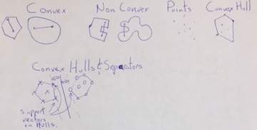
A set `C subset RR^n` is convex if for any `vec{x}, vec{y} in C` the line segment between them, `{vec{z} | vec{z} = u vec{x} + (1 -u)vec{y} mbox( where ) u in [0,1] }`, is also in `C`.
Given a set of points `X subseteq RR^n`, the convex hull of `X`, `conv(X)`, is the smallest convex set which contains `X`. Since `RR^n` is convex and contains `X`, and since the convex sets containing `X` can be partially ordered by inclusion, we know `conv(X)` exists.
When `X` is finite, say because it comes from either the positive or negative examples of training task, then `conv(X)` will be:
`{w | w = sum_{i=1}^k a_i vec{x}_i, 0 le a_i, sum_{i=1}^k a_i = 1, mbox( where each ) vec{x}_i in X}.`
In the finite case, usually only some of the points in `X` will be on the boundary of convex hull and the rest will be interior to it. The points in `X` on the boundary of `conv(X)` in 2D form a polygon. When we give an algorithm for convex hulls we are usually asking to find the points in `X` on the boundary of the hull, as these suffice to determine the set of interior points.
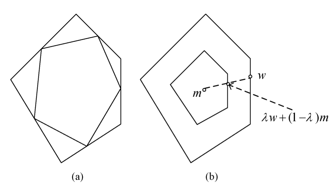
For a finite set of points `X subset RR^n` and `mu < 1`, we define the `mu`-reduced convex hull of X, `R(X, mu)`, to be:
`{\vec{w} | \vec{w} = sum_{i=1}^k a_i vec{x}_i, 0 le a_i le mu, sum_{i=1}^k a_i = 1, mbox( where each ) \vec{x}_i in X}.`
For a set of `k` points `X ={vec{x}_1, ..., vec{x}_k} subset RR^n`, let `vec{m}=1/k sum_{i=1}^k vec{x}_i` be its centroid and let `lambda le 1`. We define the `lambda-`scaled convex hull of X, `S(X, lambda)`, to be:
`{\vec{w} | \vec{w} = \lambda sum_{i=1}^k a_i \vec{x}_i + (1 - lambda)m, 0 le a_i le 1, sum_{i=1}^k a_i = 1, mbox( where each ) \vec{x}_i in X}.`
From the image above we can get some intuition as to why when separating training data, the support vectors will be on the convex hull.

Remarks on Convex Hulls and Their Variants

Convex hulls have many applications in computer graphics and video game design. For example, it is often easier to determine if the convex hulls of two objects are intersecting than directly determining if the objects themselves are intersecting.
There are divide-and-conquer algorithms for computing convex hulls of a finite set of points in 2 and 3-dimensions which run in `O(n log n)` (See O'Rourke 1998): Roughly, sort the points by their `x` coordinate. Put first half of the points in one set, the rest in the other. Compute convex hulls of the two sub-problems and merge results).
Given this, one strategy to find the maximal separator one might take is:
1. Compute the convex hull of the the positive training examples, `conv (X^+)`.
2. Compute the convex hull of the the negative training examples, `conv (X^-)`.
3. Find the nearest points on the two hulls and consider the line segment/plane between them.
4. Return the perpendicular bisector as the maximal margin separator.
In 2 or 3 dimension the run time of the above can be shown to be `O(n log n)`. To handle non-separable training data one could then use either the reduced or scaled convex hulls.
The above figure shows an examples of an original hull and interior to it on the left a `mu={1/2}`-reduced convex hull and on the right a `lambda={1/2}`-scaled convex hull. As we can see the scaled hull better retains the shape of the original figure and this gives some of the reason why it might be preferable.
In higher dimensions, the typically greater than three inputs to an SVM situation, just writing out convex hulls can be time prohibitive (facets on `d`-dimensional hulls will typically involve `d` many points chosen as a subset of all the points in `X`). A lower bound of time `n^{lfloor d/2 rfloor}` is known (Klee 1980), with the best algorithms running in time `O(n log n+ n^{lfloor d/2 rfloor})`.
So in higher dimensions we want to follow the geometrically nice approach like the above, but avoid computing complete convex hull. Instead, if we know the convex hulls `conv (X^+)` and `conv (X^-)` can be separated, we want to use surrogates for the whole hull such as nearest point algorithms between hulls.

SVMs

Outline

Introduction

Computing Separators

Popular Choices of Kernels

Iterative Algorithms for Maximal Separators

Convex Hulls and Their Variants

Remarks on Convex Hulls and Their Variants

In-Class Exercise