Introduction

Last week, we began considering strengths and weaknesses of single layer perceptron networks.
We gave a simple proof that a single preceptron cannot compute the XOR function.
We then began working towards Minsky and Papert's 1969 result concerning two layer networks and parity.
Towards this result, we showed (recall `#(vec{x})` counts the number of on bits in a bit-vector):
Lemma. Suppose a symmetric function `f(vec{x})` is computed as `|~ vec{w}\cdot vec{x} \geq theta ~|`, where `vec{w} in RR^n` and `theta in RR`. Then there exists a `gamma in RR` such that `f(vec{x}) = |~ gamma cdot #(vec{x}) \geq 1 ~|` for all `vec{x} in {0,1}^n`.
We pick up our discussion with a statement of Minsky Papert (1969)...

Minsky Papert (1969)

Theorem . Let `Psi_k^n` be the collection of all boolean functions computable by perceptrons on `n` inputs which depends on exactly `k` of these inputs being 1. Then if `K < n`, `PAR_n` cannot be computed as `|~sum_{j=0}^K sum_{psi_{jk} in Psi_j^n}[alpha_{jk} psi_{jk}(\vec{x))] \geq 1 ~|`

Remark: There are potentially a lot of functions `psi_{jk} in Psi_j^n` so the inner sum is potentially exponential size in `n`.

Proof. Suppose `PAR_n` could be computed as above. Notice if `psi_{jk}` and `psi_{jk'}` depend on the same inputs being 1, we could combine their contribution to top level pereceptron as `(alpha_{jk} + alpha_{jk'}) psi_{jk}(\vec{x})`. Notice given two bit vectors, `vec{x} ne vec{x'}` which have exactly `j` many `1` bits on, `PAR_n(vec{x}) = PAR_n(vec{x'})`. In the first case, `|~sum_{j=0}^K sum_{psi_{jk} in Psi_j^n}[alpha_{jk} psi_{jk}(\vec{x))] \geq 1 ~|` reduces to at most one `j`th level summand `alpha_{jk} psi_{jk}(\vec{x)) ` and in the second case `alpha_{jk'} psi_{jk'}(\vec{x'))` and they have to agree. This shows we can take the coefficients for a given `j` level all to be the same. I.e., `alpha_{jk} = alpha_{jk'}`. Hence, our formula above can be simplified to `|~sum_{j=0}^K alpha_{j } [sum_{psi_{jk} in Psi_j^n} psi_{jk}(\vec{x))] \geq 1 ~|`.

`sum_{psi_{jk} in Psi_j^n} psi_{jk}(\vec{x)) = N_j(vec{x})` where `N_j(\vec{x})` is the number of subsets of `vec{x}` with exactly `j` many inputs 1. So `N_j(\vec{x}) = ((#(\vec{x})),(j))`,a polynomial degree `j` in `#(\vec{x})`. Hence, our formula for `PAR_n(vec{x})` reduces to `|~sum_{j=0}^K alpha_{j } ((#(\vec{x})),(j)) \geq 1 ~|`. Pulling the 1 to the other side of the equation, determining the output of this inequality can be viewed as checking if a polynomial of degree at most `K` in `#(\vec{x})` is `\geq 0`. Notice when `#(\vec{x}) = 0`, this polynomial needs to be less than `0`, when `#(\vec{x}) = 1`, it must be at least `0`, etc. So it needs to cross the a line just below the `x`-axis at least `n` times. Therefore, by the fundamental theorem of algebra, its degree `K` must be at least `n`. Q.E.D.

Quiz

Which of the following is true?

`\P\A\R_3` can be computed by a four neuron Perceptron network.
Python does not support multiple inheritance.
xrange is a Python3 function.

On the Power of Perceptron Networks

We recall again if we are going to be able to learn a function `f` using a network of perceptrons of a particular architecture, then `f` better be computable by this network for some choice of weights.
So let's try to get a handle on the kinds of things computable by simple networks of perceptrons.
To start let `k >0` be an integer, define
`T_{k}^n(x_1, ..., x_n) = |~sum_i x_i \geq k~|` (at least `k` of the inputs must be on)
and define
`bar{T}_{k}^n(x_1, ..., x_n) = |~sum_i -x_i \geq - k~|` (at most `k` inputs 1).
We'll call these functions threshold gates.
These functions are very nice special kinds of perceptrons as all the weights are the same.
An interesting particular type of threshold gate is the majority gate:
`MAJ_n(x_1, ..., x_n) = T_{\lfloor(n)/2\rfloor +1 }^n(x_1, ..., x_n)`
Majority is 1 when most of its inputs are 1. I.e., you can think of it as like a voting gate.
A two layer network consisting of majority gates could compute functions like our electoral college system in the U.S. does. It is not surprising such networks turn out to be strictly more powerful than single layer networks.

Facts About Threshold Functions

`T_{k}^n(x_1, ..., x_n) = T_{k}^n(x_{pi(1)}, ..., x_{pi(n)})` and `bar{T}_{k}^n(x_1, ..., x_n) = bar{T}_{k}^n(x_{pi(1)}, ..., x_{pi(n)})` for any permutation `pi`.
`vv_{i=1}^n x_i = T_{1}^n(x_1, ..., x_n)`
`^^_{i=1}^n x_i = T_{n}^n(x_1, ..., x_n)`
`neg x = bar{T}_{0}^1(x)`
`^^_{i=1}^n (neg x_i) = bar{T}_{0}^n(x_1, ..., x_n)`
By repeating inputs, arbitrary positive integer weighted inputs can be computed using a threshold function.
`^^_{i=1}^n x_i = MAJ_(2n-1)(x_1, ..., x_n, vec{0})` where `vec{0}` is `n-1` zeros.
`vv_{i=1}^n x_i = MAJ_(2n-1)(x_1, ..., x_n, vec{1})` where `vec{1}` is `n-1` ones.

Conjunctive and Disjunctive Normal Form

A literal, `l_i`, is used to mean either a variable `u_i` or its negation `neg u_i`. We often write `neg u_i` as `bar u_i`.
A formula is said to be in conjunctive normal form, (CNF), if it is AND of ORs of variables or their negation.
For example, `(u_1 vv bar u_2 vv u_3) ^^ (u_2 vv bar u_3 vv u_4) ^^ (bar u_1 vv u_2 vv bar u_4)`
We often write CNF formulas like `^^_i(vv_j nu_(i_j))`
`vv_j nu_(i_j)` are called clauses.
A formula is said to be in disjunctive normal form, (DNF), if it is OR of ANDs of variables or their negation.
For example, `(bar u_1 ^^ u_2 ^^ u_3) vv (baru_2 ^^ bar u_3 ^^ u_4) vv (bar u_1 ^^ u_2 ^^ bar u_4)`
We often write DNF formulas like `vv _i(^^_j nu_(i_j))`.

CNFs and DNFs are universal

Claim. For every Boolean function `f:{0, 1}^n -> {0,1}`, there is an `n`-variable CNF formula `phi` and there is an `n`-variable DNF formula `psi`, each of size at most `n2^n`, such that `phi(u) = psi(u) = f(u)` for every truth assignment `u in {0, 1}^n`. Here the size of a CNF or DNF formula is defined to be the number of `^^`'s/`vv`'s appearing in it.

Proof. For each `v in {0,1}^n` we make a clause `C_v(u_1, ..., u_n)` where `u_i` appears negated in the clause if bit `i` of `v` is `1`, otherwise, it appears un-negated. Notice this clause has `n` ORs. Also notice `C_v(v) = 0` and `C_v(u) =1` for `u ne v`. Using these `C_v`'s we can define a CNF formula for `f` as:
`phi = ^^_(v:f(v) = 0) C_v(u_1, .. u_n)`.
I.e., we are computing an AND over the rows of the truth table which are false and computing an OR of literals which ensures this false row does not happen. As there are at most `2^n` strings `u` which make `f(u)=0`, the total size of this CNF will be `n 2^n`.

For the DNF formula let `A_v(u_1, ..., u_n)` be an AND based on the `v`th row of the truth table, where `u_i` appears negated in the AND if bit `i` of `v` is `0`, otherwise, it appears un-negated. Then we define
`psi = vv_(v:f(v) = 1) A_v(u_1, .. u_n)`. Q.E.D.

Notice either at least half of the row in the truth table for `f` are 1 or at least half of the rows are `0`. By picking the DNF in the former case and the CNF in the latter, and from our earlier results expressing ANDs and ORs using threshold gates we thus have:

Corollary. For every Boolean function `f:{0, 1}^n -> {0,1}`, there is an at most three layer network of threshold functions of size `O(n2^{n-1})` computing it.

Remark. The top threshold computes an AND or an OR of up to `2^{n-1}` rows, so has exponential size.

`p`-time algorithms

A photo an a Turing Machine implemented in real-life

When people formally try to write down polynomial time algorithms they usually give a Turing Machine (TM) implementation.
This is because TMs are a relatively simple mathematical model of computation which is capable of simulating, with less than a cubic slow-down, computations carried out on modern day computer architectures using modern day instruction sets (This result was probably shown in your undergrad automata class when presenting the Church-Turing thesis).
For the purpose of the next result, we assume a TM with 1 tape.
The tape is made up of cells each containing one of the symbols `0`, `1`, blank, $ (start-of-tape).
Only one square has the $ symbol and has one tape head is over exactly one cell at a given time.
The tape has arbitrarily many squares to the right of the $ symbol.
In one time step, a TM machine can read 1 symbol from the tape head location, write one symbol back to that location (provided that the symbol was not $), and move the tape head to the left, right, or stay put.
The action performed by the TM at a given time step is uniquely determined by its current state `q` from a finite set a states and the current symbol being read.
A polynomial time algorithm is specified by given a runtime bounding polynomial `p(n)` and the complete transition table which maps pairs `(q, \i\n_{symbol})` to triples `(q',\o\u\t_{symbol}, mbox(left-right-stay-put))`.
A computation of such an algorithm on an `n`-bit input `x_1, ..., x_n` consists of starting the machine with the tape cells given as `\$x_1x_2...x_n` and all the other cells blank. Running the machine for `p(n)` steps, and defining the output to be string given by the non-blank, non-`\$` tape cells.

Simulating `p`-time algorithms with Threshold circuits

Theorem. A `p(n)`-time algorithm for a 1-tape TM can be simulated by a `O(p(n))`-layer threshold network of size `O(p(n)^2)`. Moreover, the `O(p(n))`-layers, are built out of one layer which maps the input to an encoding of input, followed `p(n)`-many `O(1)`-layer networks each of which compute the same function `L`, followed by a layer which maps the encoding of the output to the final output . An `L` layer can be further split into `p(n)` many threshold networks each of size `O(1)` with `O(1)` inputs computing the same function `U` in parallel.

Remark. Imagine we were trying to learn a `p`-time algorithm. The result above says that we just need to learn the `O(1)` many weights in the repeated `U`, not polynomially many weights as you might initially guess. We can think of `U` as roughly corresponding to the neural nets finite control. The idea of using repeated sub-networks each of which use the same weights is essentially the idea behind convolutional neural layers.

Proof of Simulation Result

Let `|Q|` be the number of states of our polynomial time TM algorithm and let `p(n)` be the run time bound.
In `p(n)` time steps, a TM can affect at most `p(n)` many tapes cells.
We can encode the contents of a tape cell with a `3 + |~log|Q| ~|` bit number, the first bit `|~log|Q| ~| + 1` bits are `0` if the tape head is not over the square, otherwise they say the machine state. The last two bits are 00, if the tape cell has a `\$` in it; 01, if it has a 1 in it; 10 if it has a 0 in it; 11 if it is blank.
Given our result about any boolean function being computable by a depth 3 threshold function, we know we can find two fixed finite threshold networks which take a 1-bit input, either 0 or 1, and output the high and low bits of the encoding of 0 or 1.
The first layer of our network consists of a fixed finite size hard-coded circuit outputting the encoding of the pair (initial state, `\$`), saying the tape is over `\$` and the machine is in the initial state, followed by circuits which map each `x_i` to their encoding as `|~log|Q| ~| + 1` zero bits (tape head not there), followed by either 01 or 10 depending on the value of `x_i`. The remainder of the layer outputs encodings of `p(n) - n` many blank squares.
The units `U` of the intermediate layers will each take `3(3 + |~log|Q| ~|)` input bits and output `3 + |~log|Q| ~|` output bits. The `3 + |~log|Q| ~|` output bits will correspond to the encoding of a particular tape cell at one time step further into the future.
The value of this cell depends only on the values of the tape square, and those to its left and right at the current time step as well as the current state so can be computed by some fixed finite size threshold circuit.
A layer will consist of `p(n)` many such `U` circuits each having as inputs the encodings of appropriate tape squares at layer (can be viewed as time step) `t` and having as output the appropriate encodings of tape cells at layer (can be viewed as time step) t+1.
After `p(n)` many such layers the output will be an encoding of the output tape cells of the TM after `p(n)` many steps.
The final layer of our network then computes a mapping back from tape cells to a binary string. Q.E.D.

Support Vector Machines

Before we talk exclusively about deep neural networks, I want to explore one more single layer neural network architecture which is often used in machine learning: Support Vector Machines (Cortes Vapnik 1995).
An SVM computes a function `|~\sum_{j=1}^mw_j f_j(\vec{x}) ge theta~|` where `vec{f}:RR^n->RR^m`. That is, we take an input `x_1, ..., x_n`, we then map it to some different space of potentially higher dimension, and then ask if the result is above or below some hyperplane.
Often rather than taking the output to be 1 for above the hyperplane and 0 for below, we will use instead 1 for above the hyperplane and -1 for below. Both settings are of equivalent power and we will indicate as needed which one we are in.
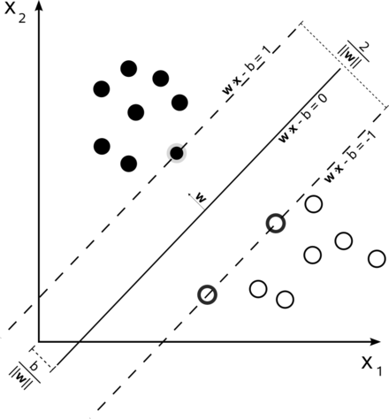
Given a training set `X`, the SVM training algorithm computes the weights `w_i` so that the separating hyperplane maximizes the distance to the nearest positive and negative training set examples. See image above from Wikipedia.
So we can see this separator is computed geometrically, rather than by an update rule.
The separating hyperplane only depends on the points closest it in the training data. When solving the optimization problem to get the hyperplane, this allows one often to avoid computing the inner product of points `vec{f}(\vec(x_j)) cdot vec{f}(\vec(x_k))` and instead compute a simpler function `k(\vec{x_j}, \vec{x_k})` called a kernel. Using a kernel, is called using the kernel trick.
Cortes and Vapnik paper extended earlier work of Vapnik and Chervonenkis (1963) and others. One of their contributions was to define a good hyperplane based on soft margins that behaves well even when the positive and negative values cannot be separated by a hyperplane.

Mapping to a Separable Space

Theorem. It is always possible to map a dataset of examples `(vec{x}, y_i)` where `vec{x} in RR^n` and `y_i in {0,1}` to some higher dimensional `vec{f}(vec{x}) in RR^m` such that the negatives examples `vec{f}(vec{x_j})` can be separated from the positive examples `vec{f}(vec{x_k})` by a hyperplane in `RR^m`.

Proof. Let `f_(vec{z})(vec{x})` be the function which is `0` if `vec{x} ne vec{z}` or if `vec{z}` was not a positive training example and is `1` otherwise. Let `vec{f}` be the mapping from `RR^n -> RR^{2^n}` given by `vec{x} mapsto (f_{vec{0}}(vec{x}), ...,f_(vec{z})(vec{x}), ..., f_{vec{1}}(vec{x}))`. All of the negative examples will map to the `0` vector of length `2^n` and a positive example will map to a vector with exactly one coordinate 1. Hence, the hyperplane which cuts each axis in the target space at a `1/2` will separate the positive from the negative examples. Q.E.D.

Corollary. Any boolean function can be computed by an SVM (maybe slightly relaxing the definition of maximally separate to allow for unbounded support vectors).

Remark. The above construction gives an SVM which does not generalize very well, so it is not really a practical construction.

Remark. For SVMs, usually `y_i`'s are chosen from `{-1, 1}`, but a similar theorem to the above could still be obtained.

Other Ways to try to Map to a Separable Space

Suppose we want to compute `PAR_2(x_1, x_2)`.
Define a mapping from `RR^2` to `RR^2` by:
`f_1(x_1,x_2) := exp(-||((x_1),(x_2)) - ((1),(0))||^2)`
`f_2(x_1,x_2) := exp(-||((x_1),(x_2)) - ((0),(1))||^2).`
We call functions `f_{\vec{t}, sigma}(vec{x}) = exp(-||vec{x} - vec{t}||^2/(2sigma^2))` where `sigma in RR`, Gaussian functions.
A function `f_{vec{t}} := phi(||vec{x} - vec{t}||)` for some function `phi: RR -> RR` is called a radial basis function.
Notice `f_1` is almost `0` except close to the vector `((1),(0))` where it approaches 1, and similarly `f_2` is almost `0` except close to the vector `((0),(1))` where it approaches 1.
Hence, an input `(x_1, x_2)` to `PAR_2` will map close to `((0),(0))` for inputs `(0,0)` or `(1,1)` and `(0,1)` will map close to `((0),(1))` and `(1,0)` will map close to `((1),(0))`.
So we can separate them with the line `1/2x + 1/2 y = 1/2`.
A function which computes an activation function on a weighted sum of radial basis function inputs is called a radial basis network.

Computing Separators

Let's consider the problem of computing the maximal separator assuming we didn't do any mapping `vec{f}`.
The standard way to do this reduces the problem to solving a quadratic program: Maximize
`mbox(argmax)_(vec alpha) (sum_j alpha_j - 1/2 sum alpha_j alpha_k y_j y_k (vec x_j cdot vec x_k))`
subject to `alpha_j ge 0` and `sum_j alpha_jy_j = 0`.
Here the weights of the output SVM are related to the `alpha_j`'s above via the equation `vec w = sum_j alpha_j vec x_j`.
A classifier can be built out of `vec alpha` directly using the equation:
`h(vec x) = sign(sum_j alpha_j y_j(vec x cdot vec x_j) - b)`
which also only uses the data in a dot product.
An important property of the `alpha_j`'s is that they are `0` usually except the support vectors -- the closest vectors to the separator (typically in each dimension).
If we want to do a mapping `vec{f}` before computing the separator, the process is almost identical, except now the classifier becomes: `h(vec x) = sign(sum_j alpha_j y_j(vec{f}(vec x) cdot vec{f}(vec x_j)) - b)`
For some `vec{f}` we can replace the `(vec{f}(vec x) cdot vec{f}(vec x_j))` in classifier and `(vec{f}(vec x_j) cdot vec{f}(vec x_k))` in the quadratic program with a simple kernel function `k(vec{x}, vec{x}_j)` or `k(vec{x_j}, vec{x}_k)`.
A result known as Mercer's theorem says when this is okay to do.

Popular Choices of Kernels

A Polynomial Kernel: `(vec{x}^Tvec{x_i} +1)^p`. Might use when we imagine in the original space it is likely we could separate the positive from the negative examples by a polynomial.
A RBF or Gaussian Kernel: `exp(-||vec{x} - vec{x_i}||^2/(2sigma^2))`. We might do clustering on the data and choose `sigma` based on the closest clusters. Then the idea why this kernel might be useful is based on parity example I gave.
A Two Layer Perceptron Kernel: `tanh(beta_0vec{x}^Tvec{x_i} + beta_1)`.
Next day, we will discuss a simpler way and more recent technique to compute the separator not based on quadratic programming.

Finish Go/No-Go Perceptron Results - Start SVMs

Outline