Outline
- HAM-CYCLE, TSP and SUBSET-SUM in NPC
- Approximation Algorithms
- Approximation Algorithm for Vertex Cover
- Quiz
- Approximation Algorithm for TSP with the Triangle Inequality
- A TSP Inapproximibility Result
Introduction
- Recall a language `L` was a set of strings over an alphabet, `A`, and a decision procedure for `L` is a procedure,
which when given a string `x` outputs "Yes", if `x in L`, and "NO", otherwise.
- `NP` is the class of languages that have polynomial time verification algorithms. That is, there is a p-time algorithm
`A(x,y)` and a polynomial `q` for each `L in NP` such that `x in L` iff `exists y \leq q(|x|)[A(x,y) = 1]`.
- We have been studying the hardest languages in `NP`, the `NP`-complete languages (NPC). `L in NPC` if `L in NP`, and for any
`L' in NP` then is a `p`-time function `f` such that `x in L'` iff `f(x) in L`.
- Thousands of problems have been shown to be `NP` complete: scheduling problems, fault detection in circuits, program optimization,
clustering, deadlock avoidance, minesweeper, etc.
- In this class, we have shown so far CIRCUIT-SAT, SAT, 3-SAT, CLIQUE, and VERTEX COVER are `NP`-complete.
- We showed CIRCUIT-SAT was in `NPC` by directly showing how to reduce an arbitrary language in `NP` to CIRCUIT SAT.
- For all the other results, we showed how to reduce a problem which we know is in `NPC` to the target language we are trying to show is in `NPC`.
- Today, we continue to show `NP`-completeness results.
Hamiltonian Cycles
- Recall a Hamiltonian cycle is a permutation of the vertices
`v_(i_1),..., v_(i_n)` of a graph `G` so that there is an edge between
`{v_(i_j) , v_(i_j+1)}` for each `j` as well an edge `{v_(i_n) , v_(i_1)}`.
- Let HAM-CYCLE be the language `{langle G rangle | G` contains a Hamiltonian cycle`}`.
Theorem. HAM-CYCLE is `NP`-complete.
Proof. First, given a permutation of the vertices, we can in
polynomial time verify whether or not it is a Hamiltonian cycle. So HAM-CYCLE is in `NP`.
To see it is `NP`-complete, we show VERTEX-COVER `le_p` HAM-CYCLE. Given a graph `G` and
an integer `k`, we need to make a new graph `G'` which has a Hamiltonian cycle iff
the original had a vertex cover of size `k`...
More NP-Completeness Proof of HAM-CYCLE
We will make use of the following widget `W_(uv)` to build a new graph `G'` from `G`:
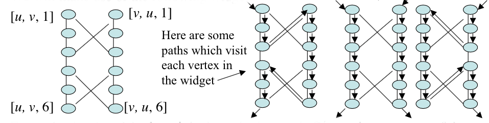
The middle path in our example paths above will be used if `u` and `v` are both in cover of `G`.
For each edge `{u, v}` in the original graph, the graph `G'` contains one copy of the widget
`W_(uv)` (i.e, `W_(uv)` and `W_(vu)` are the same widget) and we denote the edges of the widget by
`[u, v, i]` or `[v, u, i]` according to if they are on the left or right side. Only the tops and
bottoms of widgets will be connected to the rest of the graph `G'`. In our construction, a
cycle must visit each widget, and there are exactly three different ways (as shown above) one could
visit all the vertices of the widget: start on the left side, the right side, or do the two sides
separately. In addition to the vertices of the widgets, we will have selector vertices,
`s_1,..., s_k`. The edges chosen in these selector vertices will correspond to the `k` vertices of the
vertex cover in `G`. We also have two additional types of edges besides those in the widgets that
we describe on the next slide.
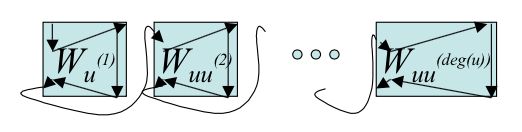
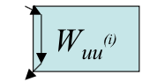
Connecting Widgets and Selector Vertices/Edges
- For each `u in V` of `G`, let `u^{(i)}` denote the vertices connected to `u` by an edge in `G`.
To `G'`, we add edges to form a path containing all widgets
corresponding to edges `{u, u^((i))}`. To do this we add the edges:
`{{[``u, u^((i)), 6``], [``u, u^((i+1)), 1``]``} | u in V}`
to `G'`. So we can construct a path from `[u, u^((1)), 1]` to `[u, u^((deg(u))), 6]` using
these additional edges.
If both `u` and `u^((i))` are in a vertex cover of `G` then we traverse a widget as
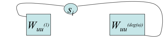
- The second kind of additional edges are of the form
`{\{s_i,[u,u^((1)) ,1]\} | u` is in `V` and `1 le i le k} cup`
`qquad {\{s_i, [u,u^((deg(u))) ,6]\} | u` is in `V` and `1 le i le k }`.
Conclusion HAM-CYCLE is NP-Complete
- If `G= langle V, E rangle` then notice the size of a widget is constant and we have `|E|` widgets.
- We also have only k selector vertices.
- Of the additional edges described on the previous slide, there are at most sum of the degrees vertices of the first type.
- There are at most `2k|V|` additional edges of the second type.
- So in all the new graph `G'` will be polynomial size in `G`.
- Suppose `G` has a vertex cover `{u_1,.. u_k}`. A Hamiltonian cycle in `G'`
can be obtained by starting at `i=1` and for each `i` thereafter follow
`s_i` to `[u_i, u_i^((1)),1]` and then the path from the previous slide to `[u_i, u_i^((deg(u_i))),6]`.
Then from there one can follow the edge `{s_(i+1), [u_i, u_i^((deg(u_i))), 6]}`. Finally,
one can following the edge `{s_k, [u_k, u_k^((deg(u_k))), 6]}` back to the start.
- Since each edge in `G` is incident with one vertex in the vertex cover each
widget will have all of its vertices hit by this path if there is cover.
- On the other hand, if there is a Hamiltonian cycle in `G'` then
`V^(star) ={ u in V | {s_j, [ u, u^((1)), 1]}` is in the cycle for some `1 le j le k}`
will be a vertex cover of size `k` in `G`.
HAM-CYCLE Reduction Example
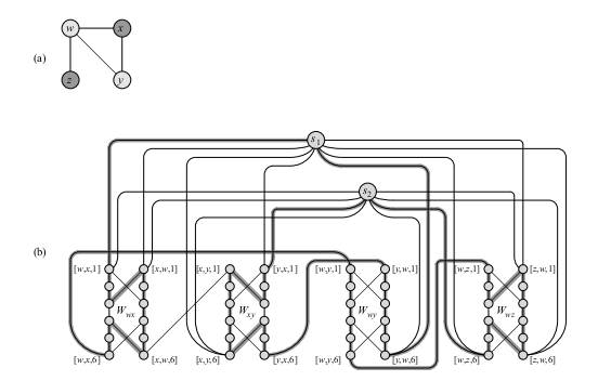
- Give the instance of VERTEX-COVER of graph (a), our reduction will produce the graph (b) (some of the
edges to and from selector vertices have not been drawn).
- The fact that the lightly-shaded vertices in (a) correspond to a vertex cover is transformed to highlighted path
in (b) which is a Hamiltonian cycle.
Traveling Salesman Problem
- In this problem a salesman must visit `n` cities. Between each pair of
cities `{i, j}` there is a cost `c_(ij)`.
- We want to know if it is possible for the salesman to see each city
exactly once (except twice for the start city) with cost less than `k`?
- TSP = `{langle G, c, k rangle | G` is a complete graph, `c` is the cost matrix,
and `k` is an integer such that the traveling salesman has a tour of cost at most `k}`.
Theorem. TSP is `NP`-complete.
Proof. First given a tour we can verify if it satisfies the desired
properties in polynomial time. So it is in `NP`. To see completeness we reduce
HAM-CYCLE to it. Given an instance `G = langle V, E rangle` of Hamiltonian cycle, we build an
instance of TSP as follows: We first let `G'` be the complete graph on the same vertices.
Then we set `c_(ij) = 0` if `{i, j}` is in `E` and `c_(ij) = 1` otherwise.
Then `langle G', c, 0 rangle` is in TSP iff `G` was in HAM-CYCLE.
SUBSET-SUM
- In the subset-sum problem we are given
a finite set `S subset NN` and a target `t in NN`.
We then ask: Is there a subset `S' subseteq S` whose elements sum to `t`?
- For example, if `S = {1,2,7, 14, 49}` and `t=16`, then the subset `S' = {2, 14}`
is a solution.
- Formally,
SUBSET-SUM = `{langle S, t rangle | exists S' subseteq S, t= sum_(s in S') s}`.
- We assume in the framing of this problem that we are encoding the numbers in binary.
NP-Completeness of SUBSET-SUM
Theorem. SUBSET-SUM is `NP`-complete.
Proof. To see SUBSET-SUM is in `NP` notice if we are given an instance `langle S, t rangle` of subset sum and
a particular encoding of set of integers `langle S' rangle`, by linear scan for each element of `S'` we can check if it is
in `S`. Further, by another scan of `S'` we can compute the sum of the elements in `S'` and then check if they are equal
to `t`. This whole procedure would take at most` O(|langle S, t rangle +langle S' rangle|^2)` and so is a polynomial
time verification procedure for SUBSET-SUM.
To show SUBSET-SUM is `NP`-hard, i.e., any language in `NP` reduces to it, it suffices to reduce 3SAT to SUBSET-SUM,
as we already showed 3SAT is `NP`-complete. Suppose `phi(x_1, ..., x_n)` is an instance of 3SAT with clauses
`C_1, ..., C_k`. WLOG, we can assume each clause has exactly three distinct literal, no clause has both a literal and its
negation, and each variable appears in at least one clause.
The reduction creates two numbers in set `S` for each `x_i` and two numbers in `S` for each `C_j`. Numbers will be
created in base 10, where each number contains `n + k` digits and each digit corresponds to either one variable or one clause.
Proof continues next slide...
NP-Completeness of SUBSET-SUM cont'd
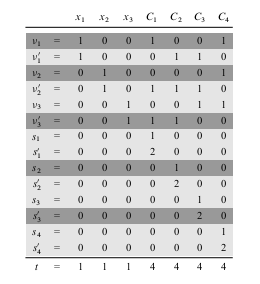
As we can see from the above picture we construct `S` and `t` by labeling each digit position by either a variable or
a clause. The least significant `k` digits are labeled by clauses, and the most significant `n` digits are labeled by
variables. In the picture above `phi = C_1 ^^ C_2 ^^ C_3 ^^ C_4`, where `C_1 = (x_1 vv neg x_2 vv neg x_3)`,
`C_2 = (neg x_1 vv neg x_2 vv neg x_3)`, `C_3 = (neg x_1 vv neg x_2 vv x_3)`, and `C_4 = (x_1 vv x_2 vv x_3)`.
- The target `t` has a `1` in each digit labeled by a variable and a `4` in each digit labeled by a clause.
- For each variable `x_i`, there are two integers `v_i` and `v'_i` in `S`. Each has a `1` in the digit labeled by `x_i` and
`0`'s in the other variable digits. If literal `x_i` appears in clause `C_j`, then the digit labeled by `C_j` in `v_i` contains a `1`.
If literal `neg x_i` appears in clause `C_j`, then the digit labeled by `C_j` in `v'_i` contains a `1`. All other digits are labeled `0`.
- For each clause `C_j`, there are two integers `s_j` and `s'_j` in `S`, Each has `0`'s in all digits other than the one labeled by `C_j`. For `s_j`, there is a `1` in the `C_j` digit, and `s'_j` has a `2` in this digit.
NP-Completeness of SUBSET-SUM Cont'd Some More
The maximum sum of digits in any digit position is at most `6`, so we don't have to worry about carries when we add numbers in `S`.
`S` contains `2n + 2k` values each with `n +k` digits, where the time to produce a digit is polynomial in `n+k`, each digit of the target can be computed in constant time, so the whole reduction from `phi` to the `S` described above is `p`-time.
Suppose `phi` is satisfiable. If `x_i = 1` in this assignment include `v_i` in `S'`; otherwise include `v'_i` in `S'`. The
sum of the `x_i` digit positions in `S'` will be `1` as we are only including one of the two `v_i`'s and all other `v_j`'s have `0` in the `x_i` digit position.
If we sum a `C_j` digit position from the elements so far added to `S'` we would get either `1`, `2`, or `3` depending on how many variables in the assignment satisfy this clauses. We can then add either `s_j` or `s'_j` or both to `S'` to ensure we get a sum of `4`.
Hence, we have shown there exists an `S'` which achieves the target.
Suppose we have have constructed `S` and `t` as above, and there is an `S'` that achieves the target sum. Then to satisfy the `x_i` digit columns we must have exactly one of `v_i` or `v'_i` in `S'`. From which we can get an assignment for `phi`. The fact that the `C_j` column sum targets were achieved will ensure this is a satisfying assignment.
Quiz
Which of the following statements is true?
- We showed in class CLIQUE is in `P`.
- There exist `NP`-hard languages which are not in `P`.
- Our proof that VERTEX-COVER is NP-complete relied on the four-color theorem.
Approximation Algorithms, Performance Ratios
-
Since it seems hard to find exact solutions to the optimization problems
associated with a given `NP`-complete problem,
it is natural to ask if one can get approximate solutions in polynomial time?
- We say an algorithm for a problem has an approximation ratio of
`r(n)`, if for any input of size `n`, the cost `C` of the solution produced
by the algorithm is within a factor of `r(n)` of the cost `C^star` of the optimal solution.
That is, `max(C/C^star, C^star/C) le r(n)`.
- We call an algorithm that achieves an `r(n)`-approximation ratio an `r(n)`-approximation algorithm.
- Some `NP`-complete problems have a trade-off between the approximation ratio and the run time.
- An approximation scheme for an optimization problem is an algorithm that takes
both an instance of the problem as well as a constant `epsilon` and then runs a
`(1 + epsilon)`-approximation on the instance.
- If for any `epsilon`, the approximation scheme run in `p`-time,
then it is called a polynomial time approximation scheme.
- We say that an approximation scheme is a fully `p`-time approximation scheme if it is an
approximation scheme and its run time is `p`-time in both `1/epsilon` and the instance size `n`.
For example, the scheme might have a running time of `O((1/epsilon)^2n^3)`.
The Vertex Cover Problem
- The optimization problem associated with VERTEX-COVER is to
find the least vertex cover of a instance graph `G`.
- The following algorithm takes a graph `G` and outputs a vertex cover
within twice the optimal.
APPROX-VERTEX-COVER(G)
1 C=∅
2 E'= E[G]
3 while E' ≠ ∅
4    let {u, v} be an arbitrary edge of E'
5    C = C ∪ {u, v}
6    Remove from E' every edge incident with either u or v
7 return C.
Analysis of APPROX-VERTEX-COVER
Theorem. APPROX-VERTEX-COVER is a p-time 2-approximation algorithm.
Proof. First, the algorithm runs in time `O(|V| +|E|)`, as we delete two
vertices and at least one edge each time through the loop.
The set `C` returned by the algorithm is a vertex cover, since each edge
that is removed is covered by some vertex in `C`. And the loop continues till
no edges left.
To see that the cover returned is at most twice the optimal,
let `A` denote the set of edges which were picked in line 4.
In order to cover the edges in `A`, any vertex cover
(including the optimal `C^star`) must include at least one endpoint of each edge in `A`.
No two edges in `A` share an endpoint, so no two edge from `A` are covered
by the same vertex from `C^star`. So `|C^star | ge |A|`. On the other hand `|C| = 2|A|`.
Approximating the Traveling Salesman Problem
- The optimization problem associated with TSP is to find a tour of least cost.
- Here is a 2-approximation algorithm for this problem
when the triangle inequality holds on the distances between cities.
APPROX-TSP-TOUR(G, c)
1. Select a vertex r to be a root vertex
2. Compute the minimal spanning tree for G from root r using Prim's algorithm
3. Let L be the list of vertices visited in a pre-order tree walk of T
4. return the Hamiltonian cycle H that visits the vertices in order L.
Subroutines used by our algorithm
- Recall in a pre-order traversal of a graph starting from some node, we visit each
child we have not yet visited, and then visit the current node.
- Recall Prims algorithm contructs a minimal spanning tree from a tree so far, denoted `A`,
which at the start of the algorithm is the empty tree.
- We maintain a priority queue of all the vertices not in A.
- The priority, `v.key`, for a vertex `v` in the queue is the least weight of any edge connecting `v` with `A`. If no such edge exists than it is `infty`.
- Let `v.pi` be the parent of `v` in the tree.
Rather than explicitly have an `A` we use this parent structure to get the tree when the algorithm terminates.
- Here is the pseudo-code:
MST-PRIM(G, w, r) // r is a starting node to grow the tree from
01 for each u in G.V
02    u.key = infty
03    u.pi = NIL
04 r.key = 0
05 r.pi = 0;
06 Q = MAKE-QUEUE(G.V) //will have all vertices
07 while Q != 0
08     u = EXTRACT-MIN(Q)
09     for each v in G.adj[u]
10        if v in Q  and u.key + w(u, v) < v.key
11            v.pi = u
12            v.key = u.key + w(u,v) //call appropriate DECREASE-KEY
Analysis of APPROX-TSP-TOUR
Theorem. APPROX-TSP-TOUR is a p-time 2-approximation algorithm
for TSP with triangle-inequality holding on the cost function.
Proof. The minimal spanning tree algorithm runs in time `O(|V|^2)`. The
remaining step take at most `O(|G|)` time.
Let `H^star` denote the optimal tour of the vertices. Since we can obtain a spanning tree
from any tour by deleting an edge, we have `c(T) le c(H^star)`
where `T` is our minimal spanning tree.
A full walk `F` of `T` lists the vertices when they are first visited and also whenever
they are returned to after a visit to a subtree. So `c(F) = 2c(T) le 2c(H^star)`. A full walk
is typically not a tour since it lists some vertices twice.
On the other, the `H` returned by the algorithm is a tour and satisfies `c(H) le c(F)`,
since it is obtained by deleting vertices from the full walk
and since the triangle inequality holds. We are using the triangle inequality as
if we have a sequence `a b c` in the full walk and delete `b`, our tour we want that the
cost does not rise.


