Outline
- Scheduling
- Brent's Theorem
- Analyzing Multithreaded Computations
- Quiz
- Parallel For Loops
The Method of Generating Functions
- Let `g(x) = sum_(i=0)^(infty) F_i x^i`. We call this power series the generating function for `F_i`.
- Consider the expression `g(x) - xg(x) - x^2g(x)`. For `i ge 2`, the coefficients will be `F_i - F_(i-1) - F_(i-2)` = 0.
- So we have:
`(1 - x -x^2)g(x) = g(x) - xg(x) - x^2g(x) = F_0 + (F_1 - F_0)x + 0x^2 + 0x^3 + cdots = x`
- This implies `g(x) = x/(1-x-x^2)`.
- Taylor expanding `x/(1-x-x^2)` and matching the coefficients with the coefficients of `g(x)` (i.e., `F_i`) gives:
`F_i = 1/sqrt(5)[((1+sqrt(5))/2)^i - ((1 - sqrt(5))/2)^i]`
- So `T(n)` of the last slide is `Theta(F_n) = Theta(phi^n)` where `phi = (1+sqrt(5))/2` and this is exponential in `n`.
- The number `phi` is known as the the Golden Ratio and it comes up all over the place in nature and
art.
Dynamic Multithreaded Fibonacci
Model of Multithreaded Execution
- We can think of a multithreaded computation as a directed acyclic graph (dag) `G= (V,E)`.
- The vertices represent instructions and the edges represent dependencies between instructions.
- An edge `(u,v) in E` means that instruction `u` must execute before instruction `v`.
- We group chains of instructions that don't contain spawn, sync, return from spawn, or parallel, into strands representing
one or more instructions.
- A strand with two successors must be followed by a spawn statement.
- A strand with multiple predecessors must be preceded by a sync statement.
- If `G` has a directed path from distinct strand `u` to distinct strand `v`, we say that the two strands are (logically) in series. Otherwise, the distinct strands
`u` and `v` are (logically) in parallel.
More on Multithreaded Execution
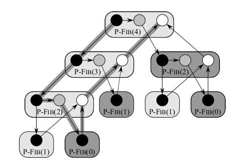
The image of the last slide shows the computation of P-Fib(4).
- Each circle represents one strand. Blacks circles are either base cases or the part of procedure up to the spawn of
P-Fib(n-1).
- Shaded circles represent the part of the procedure that calls P-Fib(n-2) up till the sync of line 5. Each group of strands belonging to the same procedure is surrounded by a rounded rectangle.
- Horizontal edges represent continuation edges, that is, an edge for execution within the same procedure
- The rectangle is lightly shaded for spawned procedures and darkly shaded for called one. A downward edge to a spawned procedure is called a spawn edge.
A downward edge to a called procedure is called a call edge. The upward edges representing the return from a spawn or call are called return edges.
- A computation starts from an initial strand, in this case, the black circle in P-Fib(4) and ends with a single final strand, in this case the white vertex in P-Fib(4).
Performance Measures
- We use the two metrics work and span to measure the theoretical efficiency of a multithreaded algorithm.
- The work of a multithreaded computation is the total time to execute the entire computation on one processor. I.e., the sum of the times taken by each of the strands.
- If we assume each strand executes in unit time, the work is just the numbers of vertices in the dag.
- The span is the longest time to execute the strands along any path in the dag.
- If we assume each strand executes in unit time, the span equals the number of vertices on a longest or critical path in the dag.
- For our graph of two slides back, if each node takes the same amount of time, then the work is 17 and the span is 8.
Runtime of a Multithreaded Computation
- The run time of a multithreaded computation depends not only on the work and the span, but also on how many processors are available and how the scheduler allocates strands to processors.
- We denote the running time of an algorithm on P processors by `T_P`.
- So work is `T_1`, the run time on one processor.
- The span is the running time if we could assign each strand its own processor. We denote it by `T_(infty)`.
- Using work and span we can get two lower bounds on `T_P`:
- Since an ideal parallel processor with `P` processors can at most do `P` units of work in one time step we have the work law:
`T_P ge T_1/P`
- A P-processor ideal parallel computer cannot run any faster than a ideal machine with an unlimited number of processors, so we have the span law:
`T_P ge T_(infty)`.
- The speedup of a computation on `P` processors is defined to be the ratio `T_1/T_P`. By the work law the speedup is always less than `P`.
- If `T_1/T_P = Theta(P)` we say the computation exhibits linear speedup, if `T_1/T_P = P`, we have perfect linear speedup.
Parallelism
- The ratio `T_1/T_(infty)` of the work to the span gives the parallelism of the multithreaded computation.
- It can be viewed as the average amount of work that can be performed in parallel along each step of the critical path.
- It upper bounds the maximum possible speedup that can be achieved on any number of processors.
- It also provides a limit on the possibility of attaining perfect linear speedup.
- To see the last statement suppose `P ge T_1/T_(infty)`. The span law implies `T_1/T_P le T_1/T_(infty) le P`. If `P >``> T_1/T_(infty)` then
` T_1/T_P lt lt P`, so the speedup is much less than the number of processors.
- As an example, consider P-Fib(4) where we assume each strand takes unit time. Then `T_1 = 17` is the time, and the span is `T_(infty) = 8`.
The parallelism is `T_1/T_(infty) = 17/8 =2.125`. So achieving much more than double speedup is impossible, no matter how many processors we use.
- We define the (parallel) slackness of a multithreaded computation on an ideal P processor computer to be the ratio `(T_1/T_(infty))/P = T_1/(P T_(infty))`.
- It represents the factor by which the parallelism of the computation exceeds the number of processors in the machine.
- If the slackness is less than 1 we cannot hope to achieve perfect linear speedup as `T_1/(P T_(infty)) lt 1` and the span law imply `T_1/T_P le T_1/T_(infty) lt P`.
Quiz
Which of the following statements is true?
- To analyze in class "How many balls fall in a given bin assuming n tosses?" we made use of the geometric distribution.
- The expected length of the longest streak in `n` tosses of a fair coin is `O(log n)`.
- In the online hiring problem if we interview `|~n/e~|` candidates and then hire the next one with a higher score than any of these, we will have more than a 50% chance of hiring the best candidate.
Scheduling
- A multithreaded scheduler must schedule the computation with no advance knowledge of when strands will be spawned or when they will complete.
That is, the scheduler must operate online.
- A centralized scheduler (as opposed to a distributed one) knows the global state of the computation at any time.
- A greedy scheduler is a centralized scheduler that assigns as many strands to processors as possible in each step.
- A complete step is a step in which at least P strands are ready to execute during a given step; otherwise, the step is incomplete.
- In a complete step a greedy scheduler assigns any `P` of the ready strands to processors.
Brent's Theorem (1974)
- The next result is a variant of a result of Brent 1974. In our context, it is due to Blumofe and Leiserson 1994.
- The work law says the best running time we could hope for is `T_P = T_1/P` and the span law says that the best running time we could
hope for is `T_P = T_(infty)`.
- The following theorem due to Brent modified for our parallel model shows that greedy scheduling is provably good in that it achieves the sum of these
two lower bounds as an upper bound.
Theorem. On an ideal parallel computer with `P` processors, a greedy scheduler executes a multithreaded computation with work `T_1` and span `T_(infty)` in
time
`T_P le T_1/P + T_(infty)`.
Proof of Brent's Theorem
We break the computation into complete and incomplete steps.
Consider the complete steps of the computation. In each complete step, the `P` processors perform `P` work. Suppose
that the number of complete steps was greater than `lfloor T_1/P rfloor`. Then the total work of the complete steps is at least
`P cdot(lfloor T_1/P rfloor + 1) = P lfloor T_1/P rfloor + P`
`= T_1 - (T_1 mod P) + P`
`> T_1`.
In the above, we are defining `(T_1 mod P) := T_1 - P(lfloor T_1/P rfloor)`, so `(T_1 mod P)` is 0 if `T_1` is divisible by `P` and is `>0` and `lt P` otherwise. The above inequality is a contradiction because this would imply that the `P` processors perform more work than the computation requires. Hence, we have
that there are fewer than `lfloor T_1/P rfloor` complete steps.
Now consider an incomplete step. Let `G` be the DAG representing the entire computation. By replacing each strand of longer than unit time computations with a chain of unit time strands, we can assume each strand takes less than unit time. Let `G'` be the subgraph of `G` that has yet to be executed at the start of an incomplete step, let `G''` be the subgraph to be executed after the incomplete step. A longest path in a DAG must necessarily start at a vertex with in-degree 0. Since an incomplete step of a greedy scheduler executes all strands with indegree 0 in `G'` the length of the longest path in `G''` must be 1 less than the longest path in `G'`. So an incomplete step decreases the span of the unexecuted DAG by 1. Hence the number of incomplete steps is at most `T_(infty)`.
Since each step is either complete or incomplete, the theorem follows.
Optimality of Greedy Scheduling
Brent's Theorem allows us to show that greedy scheduling is close to optimal in the following sense.
Corollary. The running time `T_P` of any multithreaded computation scheduled by a greedy
scheduler on an ideal parallel computer with `P` processors is within a factor of 2 of optimal.
Proof. Let `T_P^star` be the running time produced by an optimal scheduler on `P` processors. The work and span
laws give: `T_P^(star) ge max(T_1/P, T_(infty))`. Brent's Theorem on the other hand implies:
`T_P le T_1/P + T_(infty)`
`le 2 cdot max(T_1/P, T_(infty))`
`le 2T_P^(star)`. QED.
Perfect Linear Speedup versus Slackness
Our next result shows that as a computation gets more slack it gets closer to having perfect linear speedup.
Corollary. Let `T_P` be the running time of a multithreaded computation produced by a greedy
scheduler on an ideal parallel computer with `P` processors. Then, if `P lt lt T_1 / T_(infty)` , we
have `T_P ~~ T_1/P`. That is, the speedup is approximately `P`.
Proof. Suppose `P lt lt T_1 / T_(infty)`, then `T_(infty) lt lt T_1/P`. By Brent's Theorem,
`T_P le T_1/P + T_(infty) ~~ T_1/P`. As the work law says `T_P ge T_1/P`, we conclude `T_P ~~ T_1/P`. This implies
the speedup is `T_1/T_P ~~ P`. QED.
Example. Suppose the slackness, `T_1/(P T_(infty))`, was greater than 10. Then the span, `T_(infty)` term in Brent's Theorem
is less than 10% of the the work/processor term. So if a computation runs on only 10 or a 100 processors, it doesn't make sense to value parallelism, `T_1/T_(infty)`, of 1000000 over parallelism of 10000 even with the factor of 100 difference.
Analyzing Multithreaded Algorithms
- Let's analyze the P-Fib(n) algorithm.
- We showed that `T_1(n) = Theta(phi^n)` where `phi = (1+sqrt(5))/2`.
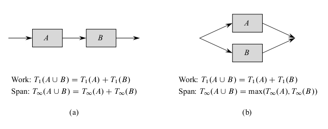
- The above diagram shows how to determine the span of a parallel computation DAG: Namely,
if two subcomputations are joined in series, their spans add to form the span of their composition; if
two subcomputations are joined in parallel, the span of their composition is the maximum of the spans of the two subcomputations.
- For P-Fib(n), the spawned call to P-Fib(n-1) runs in parallel with the call to P-Fib(n-2).
- So we can express the span of P-Fib(n) via the recurrence:
`T_(infty) (n) = max(T_(infty)(n-1), T_(infty)(n-2)) + Theta(1)`
`= T_(infty)(n-1) + Theta(1)`
which has solution `T_(infty) (n) = Theta(n)`.
- So the parallelism of P-Fib(n) is `(T_1(n))/(T_(infty)(n)) = Theta((phi^n)/n)`. This grows exponentially as `n` gets large.
- Hence, on parallel computers with a large fixed number `P` of processors, this algorithm will exhibit nearly perfect linear speedup for modest values of `n`.


