Introduction

Last Day, we were looking at mechanisms to fairly and effectively allocate network resources.
Here resources are bandwidth of links and spaces in queues. If a resource has too much demand, it is said to be congested.
We defined `Power = mbox(Throughput)/mbox(Delay)` as an effectiveness measure for a network and we defined Jain's fairness: `f(x_1,...x_n) = (\sum_(i=1)^n x_i)^2/(n \times (\sum_(i=1)^n (x_i)^2))` as a measure of fairness.
We looked at the queuing disciplines: FIFO with tail drop, priority queuing, Fair Queuing, and weighted Fair Queuing as means to allocate queue resources.
We then looked at TCP congestion control mechanisms involving the use of a CongestionWindow parameter to determine the sender's window. Different ways we considered setting the CongestionWindow were: additive increase, multiplicative decrease (AIMD), slow start (Tahoe), Quick Start, fast retransmit and fast recovery (Reno), and TCP CUBIC.
Except for the reservation-based Quick Start, these all involved periodically making the network congested to find the correct CongestionWindow for the sender.
We then started looking at congestion avoidance mechanisms, which attempt to predict when congestion is about to happen, and reduce the rate at which hosts send data just before packets start being discarded.
Two approaches to congestion avoidance are:
1. Active Queue Management (AQM) add a small amount of functionality into the routers to assist end nodes anticipate congestion.
2. End Host Techniques attempt to avoid congestion purely from the end hosts. These are typically variants of the control mechanisms previously discussed.
On Monday, we looked at one AQM technique known as DECbit. Today, we begin with a second technique called RED.

Random Early Detection (RED) (Floyd, Van Jacobson 1993)

In this scheme a router maintains a running average of its queue lengths.
It also maintains two variables MinThreshold and MaxThreshold.
If a packet arrives and the average queue length is less than MinThreshold it just queues the packet.
If it's between MinThreshold and MaxThreshold, it drops the packet with probability `P` (the drop probability). This is called early random drop.
Otherwise, it drops the packet.
The second case causes the sender to timeout earlier than if RED was not used, and so if TCP was being employed the CongestionWindow would stabilize to a workable value without putting as much load on the network.
When RED is used, the probability `P` is a function of where between MinThreshold and MaxThreshold the average length currently is.

Computing Average Queue Length

To compute a running estimate of the average queue length, the following formula is used:
`\mbox{AvgLen} = (1 - \mbox{Weight}) \times \mbox{AvgLen} + \mbox{Weight} \times \mbox{SampleLen}`
where `0 < \mbox{Weight} < 1` and `\mbox{SampleLen}` is the length of the queue when a sample measurement is made.
In most software implementations, the queue length is measured every time a new packet arrives at the gateway. In hardware implementations, it might be calculated at some fixed sampling interval.
The value of Weight determines how many samples at a high level are needed to view the average queue length as high.
The figure above shows the average weighted length on the same graph as the instantaneous queue lengths to show the smoothing effect of this kind of weighting.

Drop Packet Pseudocode

The rules for how to handle packets mentioned a couple of slides ago can be expressed in pseudo-code as:

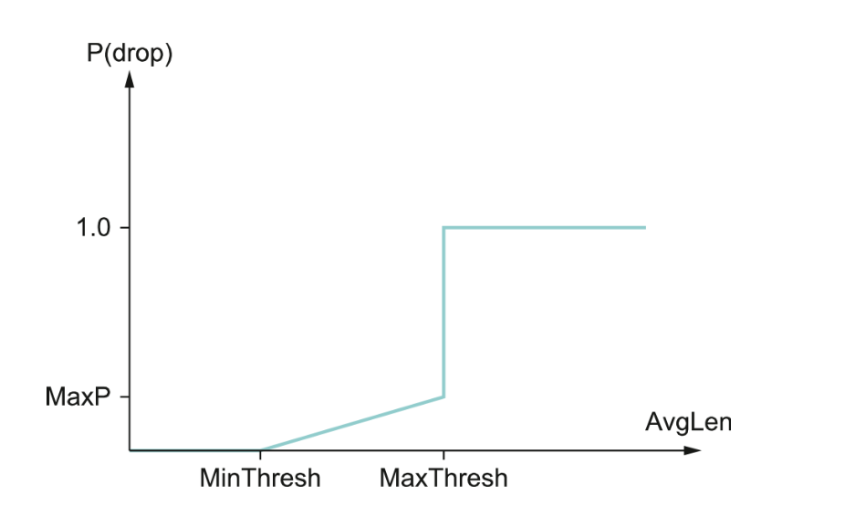
if AvgLen ≤ MinThreshold
   queue the packet
if MinThreshold < AvgLen < MaxThreshold
   calculate probability P
   drop the arriving packet with probability P
if MaxThreshold ≤ AvgLen
   drop the arriving packet

The graph above shows the probability of dropping a packet as a function of the average queue length.
When the AvgLen is between MinThreshold and MaxThreshold, the router is dropping the occasional packet to hint that senders through the router should slow down.
Notice the probability changes between MinThreshold and MaxThreshold (it isn't constant and doesn't usually go from 0 linear to 1) -- we'll say more on this on the next slide.
When the AvgLen gets above MaxThreshold, it tries to be more dramatic and drops all arriving packets to send a stronger hint.

Calculating the Drop Probability

From the previous slide, it might appear that the drop probability is only a function of AvgLen.
In fact, `P` is a function of both AvgLen and how long it has been since the last packet was dropped
It is computed as:
`\mbox{TempP} = \mbox{MaxP} \times (\mbox{AvgLen} - \mbox{MinThreshold}) / (\mbox{MaxThreshold} - \mbox{MinThreshold})`
`\mbox{P} = \mbox{TempP}/(1 - \mbox{count} \times \mbox{TempP}).`
TempP corresponds to the probabilities on the graph in the previous slide.
`\mbox{count}` keeps track of how many newly arriving packets have queued and not dropped since the last drop while AvgLen has been between `\mbox{MinThreshold}` and `\mbox{MaxThreshold}`.
So if a lot of packets have been queued and not dropped, `P` will be higher than tempP and approach 1 (if exceeds 1 or negative treat or infinite as 1). On the other hand, if a packet has just been dropped `P` will be the same as tempP.
This extra step in the calculation of `P` was added by the algorithm creators to avoid packets drops occurring in clusters.
Clustered drops are likely to occur within the same connections as opposed to be distributed across connections.
One drop per round-trip time is enough to cause a connection to reduce its window size, but multiple lost packets is likely to cause it to go back to a slow start.

Example of Calculating Drop Probability

Suppose `MaxP` is 0.02, count is 0, and the `AvgLen` is halfway between the two thresholds.
Then `TempP` and `P` would be `1/2 \times MaxP`.
An arriving packet would be added to the queue with probability 0.99.
If 50 more packets were queued without a drop, then `TempP` would be the same, but `P` would be
`0.01/(1 - 50 \times 0.01) = 0.01/0.5 = 0.02.`
If 99 packets arrived without a drop, the probability the next packet would be is:
`0.01/(1 - 99 \times 0.01) = 0.01/0.01 = 1.`
Again, if there is a drop, the count is reset to 0.

In-Class Exercise

Suppose `MaxP` were 0.03, the AvgLen was a 1/4 of the way between the two thresholds, and count was 0.
What would be the initial values for `TempP` and `P`?
Suppose 75 packets were queued in a row without a drop while AvgLen grew by a factor of 4/3 (but remained between the thresholds).
What would the new `TempP` and `P` be?
Please post your solution to the Apr 19 In-Class Exercise Thread.

Remarks on RED

The intent of RED is that if it causes the drop of a small percentage of packets when AvgLen exceeds MinThreshold, this will cause a few TCP connections to reduce their window sizes, which in turn will reduce the rate at which packets arrive at the router.
Assuming this happens, the AvgLen will then decrease, and congestion is avoided.
Queue length is averaged over time, so it is possible for the instantaneous queue length to be much larger than the average.
In this case, if the queue length exceeds the size of the queue, it might be dropped via tail drop.
One design goal of RED was to avoid tail drops as much as possible.
One interesting property of RED is that the probability that a packet is dropped for a given flow is roughly proportional to the share of bandwidth that the flow is currently getting at the router.
This is because a flow with a larger share of the bandwidth is providing more candidates to be dropped.
This property can be viewed either as entailing some kind of fair allocation, or as punishing high-bandwidth flows with a higher probability of a restart.

Setting RED Parameters

If traffic is fairly bursty, then MinThreshold should be sufficiently large to allow the link utilization to be maintained at an acceptably high level.
The difference between the two threshold should be larger than the typical increase in the AvgLen in one RTT.
Given today's mix of traffic on the internet, a common rule of thumb is to set MaxThreshold to twice MinThreshold.
One also wants that the amount of buffer space above MaxThreshold is sufficient to absorb natural bursts that occur in internet traffic without forcing the router to enter tail drop mode.
We noted previously that 100ms is not a bad estimate of average RTT between two nodes in the internet (assuming no additional information).
As it takes at least one RTT for duplicate ACKs to allow a sender to adjust its window size, it doesn't make sense for routers to respond to congestion events on timescales smaller than about 100ms.
So Weight should be chosen so that changes in queue length over time scales smaller than 100ms are filtered out.

Explicit Congestion Notification

RED relies on sending signals to TCP flows to slow down if a router is becoming congested.
A flow that ignores such signals is called an unresponsive flow.
We now look at techniques to isolate certain classes of traffic/flows from others so that they don't ignore signals and consume more than fair share of resources.
We note that if we can isolate flows, then using RED, we might drop packets from a particular flow more aggressively.
Although RED is the most extensively studied AQM, it hasn't been widely deployed because it does not result in ideal behavior in all circumstances.
Its study though motivated other approaches whereby routers send explicit congestion signals.
Instead of dropping packets as in RED, IP and TCP nowadays mark packets using an Explicit Congestion Notification (ECN) header and continue to send them on their way.
Specifically, two bits in the IP TOS field are now used as ECN bits.
One bit is set by the source to indicate that it is ECN capable. This is called the ECT (ECN-Capable Transport) bit.
The other bit (the Congestion Encountered (CE) bit) is set by the routers along the end-to-end path when congestion is encountered, as computed by whatever AQM algorithm that is running.
ECN also includes two optional TCP header flags: ECE (ECN-echo) which communicates from the receiver to the sender that it has received a packet with a CE bit set, and CWR (Congestion Window Reduced) communicates from the sender to the receiver that it has reduced its congestion window.
The actual AQM used to say when the CE bit should be set is not specified by TCP, only a list of requirements is given. We will look at these in more detail when talking about data center congestion control.

Source Based Congestion Avoidance

We now look at strategies to detect incipient congestion at the end hosts rather than at the router.
For example, a sender might guess that a router in a particular flow is becoming congested because it observes the RTTs on that flow are getting longer.
One algorithm to do this is as follows:
1. Use slow start as normal.
2. Every two RTTs, check if the CurrentRTT is greater than the average of the minimum and maximum RTTs seen so far.
3. If it is decrease the congestion window by 1/8.
A second algorithm to do this updates the congestion window every two RTTs using:
(CurrentWindow - OldWindow) × (CurrentRTT - OldRTT)
Here the windows are the sender windows. If this is positive, the sender decrease the congestion window size by an 1/8, otherwise, increase it by one packet size.
As a network approaches congestion one would expect a flattening of the sending rate.
An algorithm that uses this is: every RTT, increase the window size by 1. Compare throughput at this size to when the size was one smaller. If the difference is less than one-half the throughput achieved when only one packet was in transit, the algorithm decreases the window by one packet. Here throughput is number of bytes outstanding in the network divided by one RTT.

TCP Vegas (Brakmo Peterson 1994)

Rather than look at the flattening of the throughput, you could imagine comparing the measured throughput versus expected throughput.
This is the idea of TCP Vegas. TCP Vegas is not widely deployed yet, but the strategy it uses has been adopted by other implementations of congestion avoidance that are now being deployed.
As an example, the top graph above graphs the congestion window as earlier, the middle graph shows the average sending rate as measured at the source, and the bottom graph shows the average queue length at the bottleneck router.
Notice between 4.5 and 6 seconds the congestion window increases, but the throughput stays flat. This is because the throughput cannot increase beyond the available bandwidth. So increasing the window size beyond this point, only results in packets taking up buffer space at the bottleneck router (as seen on the bottom graph).
So if we measure the throughput we are achieving versus what we'd expect by increasing the window, we can tell when congestion is starting.
Next day, we'll look at this in more detail.

More Congestion Avoidance

Outline

Introduction

Random Early Detection (RED) (Floyd, Van Jacobson 1993)

Computing Average Queue Length

Drop Packet Pseudocode

Calculating the Drop Probability

Example of Calculating Drop Probability

In-Class Exercise

Remarks on RED

Setting RED Parameters

Explicit Congestion Notification

Source Based Congestion Avoidance

TCP Vegas (Brakmo Peterson 1994)