The next problem we will consider this semester is how to effectively and fairly allocate the resources of the Internet among a collection of competing users.
The shared resources we are worried about are the bandwidth of links and the lengths of the buffers and queues on the routers or switches where packets are awaiting transmission.
When one has too much traffic/demand on such a resource it is said to become congested.
Most networks provide some kind of congestion-control mechanism to mitigate against congestion.
Resource allocation is the process by which network elements try to meet the competing demands that applications have for their network resources.
There are three important features of the network architecture connected to resource allocation.
A given source may have more than enough outbound capacity; however, between the source and destination there may be a low capacity link or router that causes a bottleneck. This bottleneck may affect more than one route.
The sequence of packets sent between a source/destination pair following the same route is called a flow. Flows can be viewed at different granularities such as host-to-host; process-to-process.
Different networks might have different service models: such as best-effort to one in which individual flows get certain guarantees of quality of service (QoS).
Taxonomy of Resource Allocation Methods
We next look at three dimensions on which resource allocation mechanism may be classified:
Router Centric versus Host Centric -- whether it is up to routers to decide which packets to be dropped;
or whether it is the end hosts that make these kind of decisions.
Reservation-Based versus Feedback-Based -- in the first of these, resources are allocated when the flow is established; in the second way, the resources are dynamically allocated based on network conditions.
Window-Based versus Rate-Based -- allocation might be controlled by saying how big a window the hosts can have or it might be controlled by saying how many bits/second they can send.
Evaluation Criteria
In order to say how good a resource allocation mechanism is, we need to say how effectively and fairly it allocates resources.
So we need some way to define what these mean.
One way to describe the relationship between the throughput and delay of a network is the so-called power of the network:
Power = Throughput/Delay.
To effectively allocate resources we want to maximize this ratio.
One measurement of the fairness of a metric was given by Jain (1984). Given flows `1,..., n` with throughputs (`x_1,...x_n`), the fairness is defined as:
`f(x_1,...x_n) = (\sum_(i=1)^n x_i)^2/(n \times (\sum_(i=1)^n (x_i)^2)).`
This returns a value between 0 and 1 with a value of 1 if each `x_i` have the same throughputs.
The fairness so defined can be thought of as the inner product (hence, similarity) squared between a unit vector in the direction of the actual throughputs with the unit vector in the directions where all the throughputs were the same. The squaring is to avoid calculating square roots.
One can check if all the `x_i` receive 1 unit of data per second. The fairness reduces to:
`f(1, ..., 1) = n^2/(n \times n) = 1.`
One the other hand, if all received 1 unit of data per second except `x_j` which receives `1 + \Delta`, then the formula gives:
`((n-1) + 1 + \Delta)^2/(n(n-1 + (1+ \Delta)^2)) = (n^2 + 2n\Delta + \Delta^2)/(n^2 + 2n\Delta + n\Delta^2).`
So the denominator exceeds the numerator by `(n-1)\Delta^2` and the value will be less than one.
Quiz
Which of the following is true?
All stream transport protocols require in-order delivery of packets.
SUN-RPC messages are always acknowledged.
RTP's profiles and formats are an example of/can be used for application level framing.
Queuing Disciplines
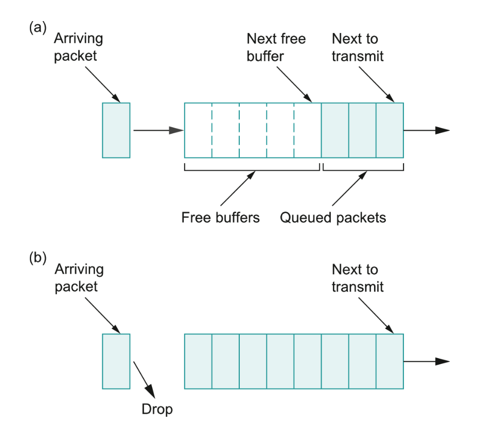
Every router must implement some queuing discipline to govern how packets are buffered while waiting to be transmitted.
This discipline can be viewed as allocating both bandwidth (saying which packets gets to
be transmitted) and allocating buffer space (which packets get discarded).
The discipline also affects the latency experienced by the packet.
We are now going to look at two queuing algorithms in terms of forwarding: first-in first-out (FIFO) and fair queuing (FQ).
FIFO Queuing
When using FIFO queuing the first packet to arrive at a router is the first to be forwarded.
It doesn't matter which flow the packet belongs to or how important the packet is.
When the queue becomes full, then the router drops incoming packets until there is more space in the queue.
This is called tail drop.
Here FIFO queuing is a scheduling policy, it determines the order in which packets are transmitted and
tail drop is a drop policy, it determines which packets are dropped.
FIFO with tail drop is the most widely used policy in internet routers today.
Notice this queuing mechanism does not take any account of congestion, so congestion mitigation has to be done on top of this.
A variation on FIFO is priority queuing. The queue is split into priority tiers using what was originally the IP Type of Service (TOS) field (now called Differentiated Services Code Point field), the first-in packet of the most important tier is sent next.
The problem with priority queuing is that the highest priority queue can starve all the other queues.
FIFO queuing doesn't differentiate between traffic sources. If priorities are being used, it doesn't police how the sources
are using the priorities.
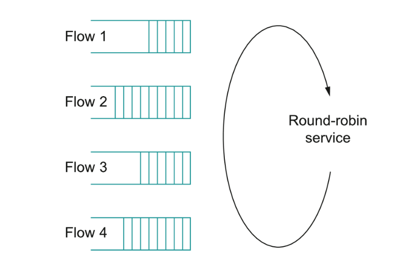
Fair queuing tries to address these issues.
It separates the queue into distinct flows being handled by the router.
The router then tries to handles the flows in a round-robin fashion.
When a queue for a given flow reaches a certain length additional packets sent to that queue are discarded.
Fair Queuing Details
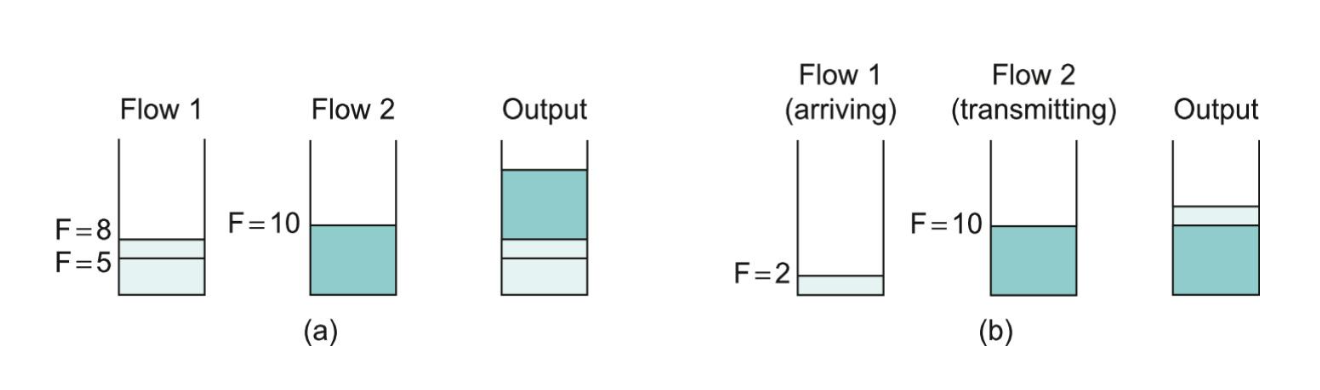
To make this more precise let `S_i` denote when the router starts to transmit packet `i`, and `F_i` denote when it finished.
Then `P_i = F_i - S_i` represents the time to send the `i`th packet.
Finally, let `A_i` denote the time the `i`th pack arrives at the router.
Then `F_i = max(F_{i-1}, A_i) + P_i`
In fair queuing, we calculate these `F_i` independently for each flow.
We choose the next packet to send as the one whose `F_i` is the lowest.
Notice this queuing discipline is work-conserving. That is, it never leaves the link idle as long as there is a least one packet in the queue.
Another thing to notice is that if the link is fully loaded and there are `n` flows, then each flow can use at most `1/n` of the total bandwidth.
A variation of FQ is weighted fair queuing. In this, each queue has a weight and we multiply the `F_i`'s by this weight and choose the lowest product as who to send next.
Fair Queuing Example
The figure above shows the queues for two flows.
In (a), fair queuing selects both packets from flow 1 to be transmitted first because of their earlier finishing times.
In (b), the router has already begun sending a packet from flow 2 when the packet from flow 1 arrives.
In this case, we don't preempt flow 2's packet, but allow it to continue to be sent, then send flow 1's packet afterwords.
TCP Congestion Control
In addition to the flow control advertised window, TCP also maintains a CongestionWindow state variable.
The equation we had for EffectiveWindow a couple lectures back is not exactly what is used in practice.
Instead, we set
MaxWindow = MIN(CongestionWindow, AdvertisedWindow), and
EffectiveWindow = MaxWindow - (LastByteSent - LastByteAcked)
Unlike the AdvertisedWindow which the receiver controls, the CongestionWindow is determined by the sender.
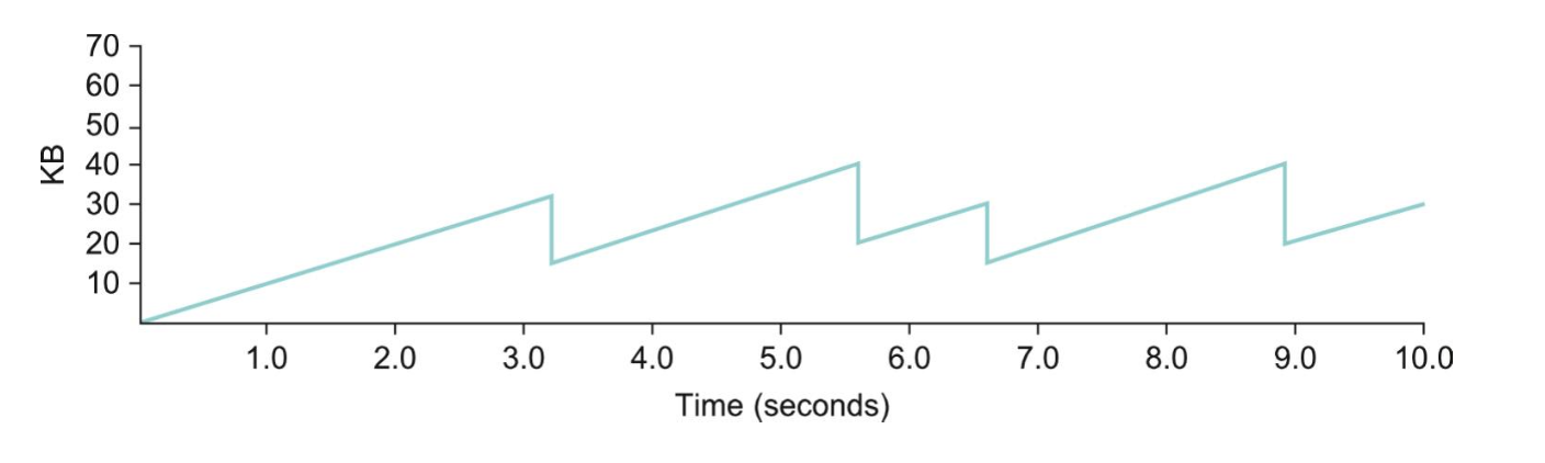
The sender tries to increase the window size when the level of congestion goes down and decrease it when it goes up. The
acronym for this is AIMD (additive increase, multiplicative decrease).
Timeouts/segment losses are used as an indication of congestion. When a timeout/loss occurs, the congestion window is halved (explaining the MD in AIMD).
The window size is not allowed to go below one MSS (maximum segment size).
On the other hand, every time TCP succeeds in sending and getting ACK's for a segment, we increase the CongestionWindow by MSS × (MSS/CongestionWindow). (This is AI in AIMD).
The reason why we add to increase and multiply to decrease is that the consequences of having a too large window (which would affect other people's traffic) are worse than those of being too small (only your traffic).
The above figure shows the typical sawtooth pattern one would expect for the CongestionWindow value as a function of time.
Slow Start (van Jacobson 1988 (called Tahoe))
The names Tahoe, Reno, Las Vegas, etc. for TCP Congestion mechanisms come from the version of BSD in which they were first implemented.
Additive increase works well, when the source is operating at close to the available capacity of the network.
It takes too long to ramp up a connection when it is starting from scratch.
TCP allows for a second mechanism called slow start to solve this problem.
The name slow start comes by comparison with how the EffectiveWindow is computed without any congestion control.
In slow start, when a connection is first set-up the CongestionWindow is set to one MSS.
After the first ACK, it doubles to 2 MSS's, then 4, etc.
When a packet loss occurs, the window is halved. This window size is called the CongestionThreshold .
So we were able to transmit okay at CongestionThreshold but not at 2 × CongestionThreshold.
We reset CongestionWindow to 1 MSS.
We then do increases based on 1, 2 ,4, etc. MSS's. When we reach the original CongestionWindow + CongestionThreshold size
we resume doing only additive increases.
If we ever time out, the CongestionWindow is set as new CongestionThreshold and then we do the above again.
and repeat.
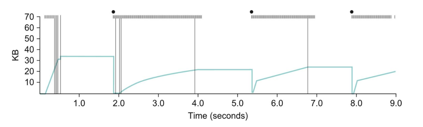
Slow Start Example
The above figure illustrates how TCP's CongestionWindow increases and decreases over time if slow start is in use.
In the above, the green line is the CongestionWindow size, hashes at the top indicate when packets were transmitted, long
lines indicates a time when a packet that was not acknowledged was sent, solid dots indicate timeouts.
Notice the rapid increase in the connection window at the start of the connection, corresponding to the initial slow start phase.
At about 0.4s, a bunch of packets are now acknowledge so the congestion window stops growing and flattens, because the sender window is full
of unacknowledged data (notice not hash marks at top during this time).
Once a timeout occurs, the CongestionWindow is reset to 1 MSS, and more packets start to be acknowledged.
Quick Start
Slow start doesn't try to estimate the available bandwidth using any information from the routers between the sender and receiver.
Quick start is one congestion control technique that tries to do this.
In quick start, the TCP sender can ask for an initial sending rate greater than slow start by putting a request in its SYN packet as a TCP option.
Routers along the path examine this option, evaluate their current level of congestion on the outgoing link for this flow, and decide if the rate is acceptable, if a lower rate should be used, or if slow start should be used.
By the time the SYN reaches the receiver, it contains a rate that is acceptable to all routers along the path, or an indication that slow start should be used.
The receiver sends this back to the sender, and in the former case, the sender thsn uses the rate to begin transmission; otherwise, slow start is used.
Fast Retransmit and Fast Recovery (van Jacobson 1990, Stevens 1994 (called Reno))
TCP timeouts are relatively course grained. As we saw, we could up with dead-air while waiting for a timer to timeout
on a lost packet.
To avoid this, a mechanism called fast retransmit was added to TCP.
When fast retansmit is being used, the receiver ACK's each packet it receives even if this is out of order. The ACK is still for the next byte expected.
This might result is several duplicate ACKs. If the sender sees three duplicates ACKs it retransmits.
Fast retransmit tends to work well when the window size is at least large enough so one can expect to see these three timeouts before the timer goes off.
Another mechanism, called fast recovery can be used to avoid having to halve the CongestionWindow on packet loss.
Rather than halving the whole congestion window. We take the average of the size that caused a problem and the Congestion Threshold.
This allows us to binary search for the correct window size.
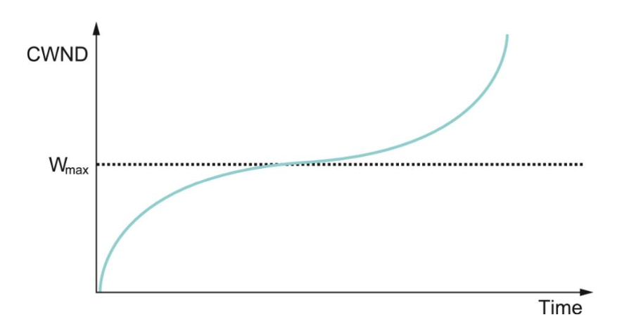
TCP Cubic
Slow start is one mechanism for updating the congestion window as a function of the last congestion event.
By default, Linux (since 2.6.13 (2006)), MacOS (since Yosemite), and Windows (Windows 10) use another mechanism called TCP CUBIC whose goal is to support networks with large delays × bandwidth products (long-fat networks).
Long-fat networks often require many-round trips to reach the available capacity of the end-to-end path.
TCP CUBIC exploits the shape of a cubic curve to more quickly return the window size to near that of the last congestion event target (`W_{max}` in the above figure).
Near the `W_{max}` size the curve is more flat (more like the additive adding), but if we pass through `W_{max}` without any further congestion issue we start increasing the congestion window size more aggressively again.
The equations for the window size with CUBIC are:
`mbox(CWND)(t) = C \times (t - K)^3 + W_{max}`
`K = (W_{max} \times (1-\beta)/C)^{1/3}`
Here `C` is a scaling constant and `\beta` is the multiplicative decrease factor. Linux uses 0.7 for `beta`.
Congestion-Avoidance Mechanisms
As described so far, TCP needs to cause congestion in the network to best find the way to consume network resources.
Alternatively, we might want to achieve the effect of using our network resources efficiently, but avoid congestion altogether.
Such a strategy is called a congestion-avoidance strategy.
DECBit
This was an early mechanism to do collision avoidance, developed by DEC.
In this scheme each router monitors the load it is experiencing and explicitly notifies the end nodes when congestion
is about to occur.
This is done by setting a binary congestion bit in the packets that flow through the router. Hence the name DECBit.
The destination host copies this bit into the ACK and when this ACK is seen by the sender it adjusts its window accordingly.
More specifically, a router sets its DECbit if its average queue length is greater than or equal to 1.
A sender increases its queue size by 1 if few than 50% of the acks it received for the last windows worth of data had the DECbit on.