On Monday, we began talking about indexes which are useful for speeding up queries on multiple columns.
These could be useful for partial match queries one might have in data cube applications or could be containment style
queries that one might have in a spatial/geographic database.
We gave two hash-based approaches to such indexes: partitioned hash tables and grid files.
We then switched to tree-like index approaches and considered multi-level indexes, kd-tree, and quad trees.
Today, we begin with another tree-based approach...
R-Trees
An R-tree node consists of a bounding region data structure (usually a rectangle), together with either pointer to child R-tree nodes,
or to the data itself (leaf case.)
R-tree can be used to store not only points, but also more complicated objects like building footprints, roads, etc.
The leaf nodes of an R-tree are supposed to have pointer to all the records that lie within the bounding region of the root.
Regions are allowed to overlap.
The algorithms used for insertion starts at the root of the tree, and grows its region if needed,
then a child is selected (often heuristically based on the child region that best holds the object)
and then the process is repeated.
If a leaf node is too full, then it is split, and the splitting is propagated back up the tree.
R-trees are useful for "Where am I?" queries: I.e., what regions in the R-tree contain a given point.
To answer such a query, we start at the root and ask if it contains the point. We then traverse the children of the
root tto see which contain the point. If a child node contains the point, we recursive search its children for containment.
Below is an example region for a node and its subregions
Bitmap Indexes
A `n`-bit vector `V` is a string of 0's and 1's of length `n`.
A bitmap index for a field `F` is a collection of n-bit-vectors, one for each value of `F`.
As an example, suppose we have a table Car with an attribute Color.
If Car had six rows, we might get a bitmap index for the different possible values for Color that
looks something like the below:
Color
Vector
red
100100
blue
010010
green
001001
A 1 above indicates that in that row of Car the given color value occurred.
So the first Car row's Color value was red, the second Car row's Color value was blue, etc.
Uses of Bitmaps
Bitmaps can be very fast for operations like intersection
and union, since these map to ANDs and ORs
They are also good for range queries.
In-Class Exercise
Suppose we have a 1000000 record table Person(ID INT AUTOINCREMENT PRIMARY KEY, Name VARCHAR(20), EyeColor INT, HairColor INT).
This table and its indexes are stored in 4096 byte blocks.
Assume INT's are represented as four bytes, record pointers are 6 bytes.
EyeColor's can take on one of three values Brown represented as 0, Blue represented as 1, Green represented as 2.
HairColor's can take on one of five values Black represented as 0, Brown represented as 1, Blond represented as 2, White represented as 3, Other represented as 4.
Estimate the number of blocks needed to have an index on both EyeColor and HairColor, if a secondary index with indirection is used, then estimate their sizes if a bitmapped index is used.
To keep it simple (but not correct) let's assume block headers take 0 bytes.
Frequently, we have lots more 0's than 1's in a given bitmap.
So it makes sense to do things like run-length encoding to compress the bitmap.
There are algorithm for doing each of the operations we mentioned on the compressed bitmaps.
Query Execution
We are going to start talking about how query results are computed by the DBMS.
An overview of the operations involved might look like:
An Algebra for Queries
One of the first steps in evaluating a query is to
turn the original SQL into an internal representation,
based on relational algebra, that we can then manipulate.
We will view our algebra as operating on bags rather than sets.
Bags (sometimes called multi-sets) are collections where order doesn't matter but where we do allow duplicates.
For example, {{1, 2, 1,3}} = {{2, 3, 1, 1}} are the same multi-set. Neither of these is the same multi-set as {{1, 2, 3}}.
We use bags since some of our operation like projecting onto attributes (columns) might result in outputs with duplicates.
Relational Algebra Expressions
Relations `R_1, R_2 ...` are expressions.
If `Q_1`, `Q_2` are an expression so are:
`Q_1 \cup Q_2`, `Q_1 cap Q_2`, `Q1 - Q2`.
`\sigma_{mbox{expr}}(Q_1)` where `mbox{expr}` is a valid selection expression.
Boolean formulas built out of things like `R.A=S.B` or `R.A=value`, `R.A ge value`, etc.
`\pi_{A_1,...A_n}(Q_1)`. (Projection) Also, allow `A_j -> A_k` to mean renaming
`Q_1 times Q_2` (Cartesian Product)
$Q_1 \bowtie_{\mbox{expr}} Q_2$ (Natural Join is a special case)
`delta(Q_1)` -- duplicate elimination on `Q_1`
`gamma_L(Q_1)` -- Grouping and Aggregate Operators applied to `Q_1`
(To handle COUNT, GROUP BY, HAVING)
`tau_L(Q_1)` -- sort `Q_1` (ORDER BY)
Expression Trees
Expression Trees are the intermediate representations of SQL queries.
There can be many equivalent expression trees for the same query.
Below is an example query, and a corresponding expression tree:
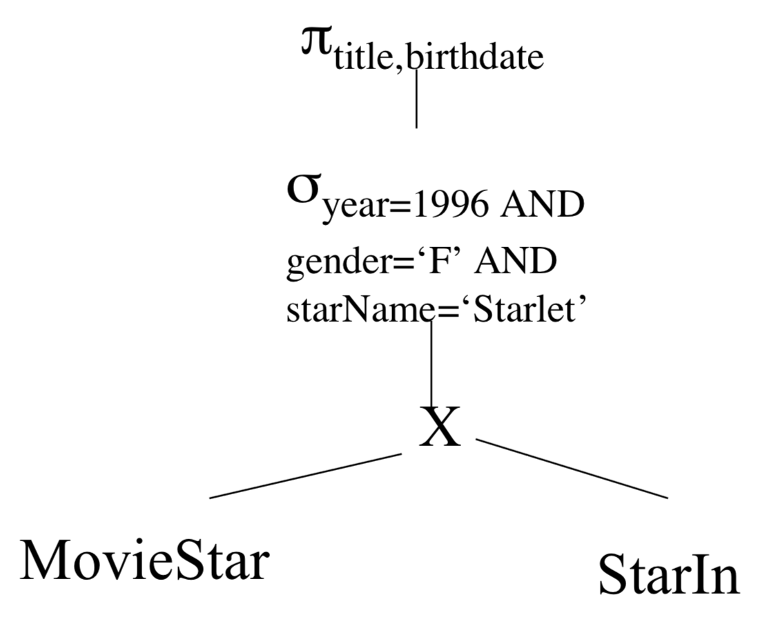
SELECT title, birthdate
FROM MovieStar, StarsIn
WHERE year =1996 AND gender='F' AND starName = 'Starlet'
Physical Query Plan Operators
Physical Query Plans are similarly built out of operators each one of which would enable us to implement a relational operator operation (or at least part of one).