Last week, we began talking about reasoning in the presence of uncertainty.
We described a Decision Theory agent which tries maximize its expected utility.
We introduced the concept of random variables
We then described how distributions on random variables can be used to come up with probability for
propositional formulas based on these variables.
Today, we begin by looking at inference in a probabilistic setting.
Probabilistic Inference
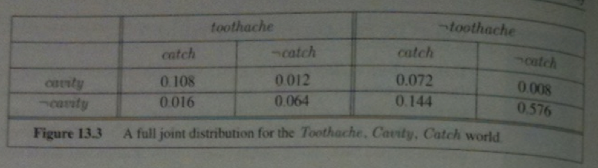
Consider a domain consisting of the three Boolean variables: Toothache, Cavity, Catch (dentist probes catches in mouth):
Notice the probabilities in the full distribution sum to 1.
There are six possible worlds in which `cavity vv t\o\othache` holds so it probability is: 0.108 + 0.012 + 0.008 + 0.016 + 0.072+ 0.064 = 0.28
Often one want to extract the distribution over some subset of variables or a single variable. For example, adding the entries in the first row gives the unconditional or marginal probability of cavity: 0.108+ 0.012 + 0.072 +0.008 = 0.2
This process is called marginalization or summing out.
The general rule for summing out any sets of variables `Y` and `Z` is:
`P(Y) = sum_(z in Z) P(Y,z).`
For example, we just calculated `\vec{P}(Cavity) = sum_(z in \{Catch, T\o\othache\})\vec{P}(Cavity,z)`.
I am writing `\vec{P}` when we are talking about the distribution rather than a proability.
If we are dealing with conditional probabilities instead of joint probabilities, we get the following rule called
conditioning: ` vec{P}(Y) = sum_z vec{P}(Y|z)P(z).
Both of these rules are useful for derivations involving probability expressions.
Example of Computing Probabilities using Conditioning
Using our definition for conditional probabilties from last day we can compute:
`P(cavity|t\o\othache) = frac(P (cavity ^^ t\o\othache) )(P(t\o\othache)) = frac(0.108 + 0.012)(0.108 + 0.012 + 0.016 +0.064) = 0.6` and
`P(neg cavity|t\o\othache) = frac(P (neg cavity ^^ t\o\othache) )(P(t\o\othache)) = frac(0.016 + 0.064)(0.108 + 0.012 + 0.016 +0.064) = 0.4`
As you expect, these sum to 1. Notice that `frac(1)(P(\t\o\othache))` appears in both of these. We can treat it as a normalization constant `\alpha` for the distribution `\vec P(Cavity |t\o\othache)` ensuring that it adds up to 1
So we can calculate `\vec(P)(Cavity |t\o\othache)` even if we don't know the value of `P(\t\o\othache)`, we just need to divide the last vector by the sum 0.12 + 0.08.
Using this we can extract a general inference procedure: Begin with the case in which the query involves a single variable, `X` (Cavity in our example). Let `\vec(E)` be the list of evidence variables (Toothache in our example). Let `vec(e)` be the list of observed values for them, and let `Y` be the remaining unobserved variables (Catch in our case). The query is `\vec(P)(X | \vec(e))` and can be evaluated as:
`vec(P)(X|vec(e)) = \alpha vec(P)(X, vec(e)) = alpha sum_vec(y) vec(P)(X,vec(e),\vec(y))`
Given the full joint distribution, this equation can answer probabilitics queries for discrete variables. It doesn't scale though: It require a table of `O(2^n)` size and so it take `O(2^n)` time to compute.
Quiz
Which of the following is true?
Composite Objects are typically modeled in Knowledge Representation systems using unit functions.
A random variable can output values bigger than 1.
One can reason about time intervals in the event calculus
Independence
Suppose we added to our three variables a fourth variable Weather to get the full joint distribution
`vec(P)(T\o\othache, Catch, Cavity, Weather)`. This table now has `2 times 2 times 2 times 4 = 32 entries`, four "editions"
of the table of the earlier slide one for each kind of weather.
What relationship do these editions have to each other and to the original three-variable table?
For example, how are `P(t\o\othache, catch, cavity, cloudy)` and `P(t\o\othache, catch, cavity)` related?
Using the product rule we know:
`P(t\o\othache, catch, cavity, cloudy) = P(cloudy | t\o\othache, catch, cavity) P(t\o\othache, catch, cavity)`
It is likely that the weather does not influence the dental variables. So it is safe to say:
`P(cloudy | t\o\othache, catch, cavity) = P(cloudy)`.
A similar equation exists for every entry in
`\vec(P)(T\o\othache, Catch, Cavity, Weather)` so we get:
`\vec(P)(T\o\othache, Catch, Cavity, Weather) = \vec(P)(T\o\othache, Catch, Cavity)\vec(P)(Weather)`
This property is called independence. In our case, the weather is independent of our dental problems
Independence means a full joint distribution can often be factored into separate disjoint distributions. Independence can
often help reduce the size of the domain representation and complexity of the inference problem.
Baye's Rule and Its Use
We already defined the product rules: `P(a ^^ b) = P(a | b)P(b)` and `P(a ^^ b) = P(b | a)P(a)`.
Equating the two right hand sides gives us:
`P(b|a) = frac(P(a|b)P(b))(P(a))`
This is called Baye's rule.
Baye's rule is used quite often in AI systems. The reason is that although `P(b|a)` might be hard to directly calculate the three terms on the right are often easier to determine
For example, we want to know the most likely cause of some effect. We could consider each cause and estimate:
`P(cause | effect) = frac(P(effect|cause)P(cause))(P(effect)).`
`P(effect | cause)` quantifies the relationship in the causal direction, whereas `P(cause | effect)` describes the diagnostic direction.
For example, a doctor often knows `P(symp\t\oms | disease)` but wants to calculate the disease that is causing the symptoms.
So if the doctor knows that 70% of people with meningitis have stiff necks and the odds of meningitis are 1/50000 and the odds
of a stiff neck are 1/100. Then the odds of meningitis given a stiff neck are (.7 * 1/50000)/0.01 = 0.0014.