Outline

• Perceptron Learning
• Feed-Forward Networks Learning

Introduction

• On Monday we began talking about neural nets.
• We said these were built-up of units. To calculate a unit takes the activations on its input lines, computes a weighted sum of these, then applies a real-valued function `g` to get a value. This value might then be fed into zero of more other units.
• We said `g` is typically chosen to be a threshold function, in which case, the unit is called a perceptron.
• We talked about recurrent (ones with feedback loops) versus feed-forward networks of units.
• The above image shows a single layer of perceptrons on the left and a multi-layer network with so-called hidden layers which are not connected to inputs or outputs directly.
• Today, we will begin by talking about learning in the single perceptron networks then look at the general feed-forward case.

Perceptron Learning

• A network with all the inputs connected to units whose outputs are the final outputs is called a single-layer neural network, or a perceptron network.
• The left image on the previous slide is an example.
• If we want to compute a function whose output is an `n` bit number with such a network, we would need to use one preceptron unit for each output.
• So to understand the power of perceptron networks, it suffices to understand what boolean-valued function a single perceptron is able to compute.
• Suppose we had two inputs `x_1` and `x_2` with activations `a_1` and `a_2`. Then the first operation we use to compute the output of the perceptron is to compute a weighted sum of the inputs `w_(00) + w_(10)a_1 + w_(20)a_2`. Recall `w_(00)a_0` where `a_0` was always 1 was a dummy input line.
• Applying a threshold at some number `t`, says when `w_(00) + w_(10)a_1 + w_(20)a_2 ge t` have the output be one value (say 1) and otherwise have it be another value (say 0).
• Notice `w_(00) + w_(10)a_1 + w_(20)a_2 = t` for fixed `t` and `w_(i0)`'s is the equation of a line in the `a_i`'s.
• Such a line could be used to separate the 0 and 1 output values of an AND or OR function as we see in the above image, but it could not be used to separate the 0 and 1 output values of the parity (XOR) function.
• In general, perceptron networks can only learn linearly separable functions.

Perceptron Networks compared to Decisions Trees

• Consider the majority functions. It returns 1 if the majority of its inputs are 1 and 0 otherwise.
• The left image above shows the training set size versus the proportion of correct answers on a test set for both decision trees and perceptrons learning this function.
• As we can by this example, with a smaller training set, the perceptron network was able to learn this function better than using decision trees.
• So there are still some reasons why we might be interested in studying perceptron learning.
• The right image above, shows a problem where decision trees do better (the will wait for a seat a restaurant problem). This is closer to a parity function.
• In any case, we are interested in how to learn the weight we should use in a perceptron network.
• This will also serve to help understand the general feed-forward case.

Sigmoid Perceptron

• Recall before we said that the activation function `g` is often taken to be a threshold function or a logistic function.
• The logistic function or sigmoid curve is defined as: `Logistic(t) = frac(1)(1+ e^(-t))`.
• We can see it plotted above.
• Notice it is very similar to a threshold function, but has the virtue of being differentiable.
• We can view the sum that we compute when trying to find the value of a perceptron as being the dot product: `vec(w) cdot vec(x)`. For now, we'll abuse notation and conflate `vec(x)` with the activations `vec(a)`.
• A sigmoid perceptron (as a function) with weight vector `vec(w)` then can be defined as
  `h_(vec(w))(vec(x)) = Logistic(vec(w) \cdot vec(x)) = frac(1)(1+ e^(-vec(w) \cdot vec(x)))`

Learning the Weights of a Sigmoid Perceptron

• Recall a training set `E` consists of examples of the form `(vec(x), y)` where `vec(x)` are the inputs and `y` is the output (0 or 1).
• The process of fitting the weights of our logistic perceptron to this example set is called logistic regression.
• The error or loss that a `h_(vec(w))` makes on the training set `E` can be calculated as:
  `Loss(vec(w)) = sum_((vec(x), y) in E)(y - h_(vec(w))(vec(x)))^2`
• Squaring is our cheap way of ensuring we are always adding nonnegative numbers.
• We want to make this function of `vec(w)` as close to 0 as possible.
• Recall one way to find the zeros of a function `f(x) = y` is to start with an initial guess of `x_0`, compute the tangent line to `(x_0, f(x_0))`, see the value `x_1` where that intersects the `x`-axis, and use that as a guess for the zero, and repeat if it is not yet close enough. Under reasonable conditions this will eventually converge on a zero.
• We want to take the same approach with the loss function above.

Learning the Weights Continued

• To compute where the tangent hyperplane hits the axis to do our steepest descent method we need to compute the gradient of the Loss function.
• Let `g` be the logistic function and `g'` its derivative.
• For a single example (term in the Loss sum), the `i`th component of the gradient is:
  `frac(del)(del w_i)Loss(vec(w)) = frac(del)(del w_i)(y - h_(vec(w))(vec(x)))^2`
  `\quad = 2(y - h_(vec(w))(vec(x))) times frac(del)(del w_i)(y - h_(vec(w))(vec(x)))`
  `\quad = -2(y - h_(vec(w))(vec(x))) times g'(vec(w) cdot vec(x)) times frac(del)(del w_i) vec(w) cdot \vec(x)`
  `\quad = -2(y - h_(vec(w))(vec(x))) times g'(vec(w) cdot vec(x)) times x_i`.
• One can verify that the derivative of the logistic function satisfies `g'(t) = g(t)(1- g(t))`.
• Substituting this into the last line above gives us an update rule for weight `w_i`:
  `n\ewW_i := w_i + alpha (y - h_(vec(w))(vec(x))) times h_(vec(w))(vec(x))(1 - h_(vec(w))(vec(x))) times x_i.`
• So to compute the weights of our perceptron, we start with an initial guess of each of the `w_i`'s. Then for each `i` and each training set item `(vec(x), y)` we calculate a `n\ewW_i` based on the weights so far. These `n\ewW_i`'s become the `w_i`'s for the next training example considered. We go through the whole training set in the way. If the values of the weight seem to be still fluctuating we run through the training set again until we get the desired/achievable stability.

Feed-Forward Networks

• Before we discuss how to do learning in feed-forward networks, let's look at how feed-forward networks can compute more complicated functions than perceptron networks.
• Recall a sigmoid perceptron layer will generally split one's space by a hyperplane into a "low" region with values close to 0 and a "high" region with values close to 1.
• We could imagine combining two thresholds one a value `t` which causes a transition from low to high with another threshold `t' > t` which causes a transition from high to low (weights would be opposite sign of the first one). This would give a network with a ridge as seen in the image above on the left.
• Combining two more perceptrons function with perpendicular hyperplanes gives a spike as seen on the right. So in at most four layers we can build a spike.
• Combining spikes allows us to compute whatever surface/function we want.

Feed-Forward Learning

• To learn with feed-forward networks we want to use the same sort of gradient descent method we used in perceptron learning.
• In order to see how this will work, lets look at the outputs of the multilayer neural net given on the first slide.
• As an example,the output activation for unit 5 can be calculated as
  `a_5 = g(w_(05) + w_(35)a_3 + w_(45)a_4)`
• We can in turn expand `a_3` and `a_4` to get:
  `a_5 = g(w_(05) + w_(35)g(w_(03) + w_(13)x_1 + w_(23)x_2) + w_(45)g(w_(04) + w_(14)x_1 + w_(24)x_2))`
• In other words, any output value can by be rewritten as function of only the input values.
• Unfortunately, this function can be highly nonlinear, so computing how the Loss affects an individual gate is harder.
• In general our algorithm will now be a kind of nonlinear regression.

More Feed-Forward Learning

• The basic strategy to train is to calculate an update from the loss function as we did in the perceptron case.
• We note the loss functions is additive, so for any weight `w` we have:
  `frac(del)(del w)Loss(vec(w)) = frac(del)(del w)||\vec(y) - vec(h)_(vec(w))(vec(x))||^2 = frac(del)(del w)sum_k(y_k - a_k)^2 = sum_k frac(del)(del w)(y_k -a_k)^2`
  where `a_k` are the activations at the last layer.
• Note given the inputs we can exactly calculate these `a_k` by expanding as on the last slide.
• The above equation shows as in the perceptron network case, if we have `m`-outputs we can decompose the problem into `m` learning problems, one for each output.
• The errors at the output layers as a function f are reasonably clear (same as the perceptron case), but how do we calculate the error for an internal unit.
• We describe how to do this for the layer immediately before the output layer. This process can then be done in the same fashion for each earlier layer back to the inputs. This process is called back propagation.
• Let `Err_k` denote the `k`th component of the vector `vec(y) - vec(h)_(vec(w))` of the last layer.
• Let `i\n_k` denote the specific value of the dot product of the weights and inputs into node `k` (again computable by expansion).
• We define the modified error to be `Delta_k = Err_k times g'(i\n_k)`. Using this, the update rule for the `j`th weight going into `k`th component of the last layer is:
  `n\ewW_(jk) = w_(jk) + \alpha times a_j times Delta_k`.
• Hidden node `j` in the layer immediately before the last layer is "responsible" for some fraction of the error `Delta_k` in each of the output nodes it connects to.
• So we divide the `Delta_k` values according to the strength of the connection between the hidden node and the output node to compute a value for `Delta_j` which could be used to then update the weights going into node `j`.
• The formula for `Delta_j` is
  `Delta_j = g'(i\n_j)sum_kw_(jk)Delta_k`.
  This formula is the error back propagation.

Back Propagation Learning Algorithm

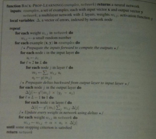
Putting this all together we get the following algorithm:

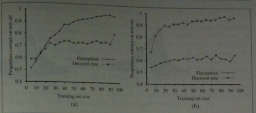
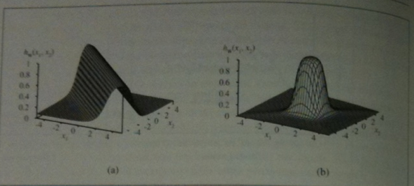
The book has a graph showing that decision tree learning in the restaurant example is only slightly better than using a feed-forward network.