Last day, we started talking about learning theory.
We then focused on supervised learning and started talking about decision trees
as a simple example where we have a learning algorithm.
We narrowed this further with decision trees with boolean values for leaves.
We then gave this learning algorithm (make me go to last day's slide)
There was one thing missing though in actually being able to implement it: implementing the
Importance function.
This says which attribute is the most important amongst those remaining to test.
Today, we first look at how to choose this attribute then we begin discussing neural nets.
Choosing the Attribute to Test
Our greedy search algorithm is designed to approximately minimize the depth of the final decision.
When it comes to pick the next attribute to test, we would like to pick the attribute that goes as far as possible toward providing an exact classification of the examples.
A really "good" attribute divides the examples into sets, each of which are all positive or all negative
examples and so will be leaves of our decision tree.
A "bad" attribute leaves the example sets with roughly the same proportion of positive or negative examples.
For example, if we are trying to decide whether to wait for a seat at a restaurant. The number of Patrons might be a good attribute, but the type of the restaurant might be a bad attribute.
To quantity "goodness" we need to define a notion of information gain.
Information Gain
Information gain is defined in terms of entropy, the fundamental quantity in information theory.
Entropy is a measure of the uncertainty of a random variable; acquisition of information corresponds to a reduction in entropy.
For example, a random variable with only one value -- a coin that always comes up heads -- has no uncertainty and this its entropy is defined as zero; thus, we gain no information by observing its value.
On the other hand, a two-sided fair coin gives one bit of information if we know its value; a pair of coins gives two bits of info, etc.
What about an unfair coin? Suppose one had a coin that was heads 99% of the time, tail 1%. Knowing that it is heads only gives us a little bit of information; but, knowing that it is tails, gives us a fair bit more.``
Entropy
The entropy of a random variable is defined as:
Entropy:
`H(V) = sum_(k)P(v_k)log_2frac(1)(P(v_k)) = - sum_(k)P(v_k)log_2P(v_k)`.
We can view this as the expected number of bits of information we will learn.
For a fair coin we have:
`H(Fair) = -(0.5 log_2 0.5 + 0.5 log_2 0.5) =1
For the 99% loaded coin, we get
`H(Loaded) = -(0.99 log_2 0.99 + 0.01 log_2 0.01) approx 0.08 bits`
Since we are interested in Boolean random variables, we will define this special case as:
`B(q) = -(qlog_2 q + (1-q) log_2(1-q))`.
For example, `H(Loaded) = B(0.99) approx 0.08`.
One can plot this function, finds its maximum (is at 1/2), etc.
Choosing a Attribute Revisited
If a training set has `p` positive examples and `n` negative examples, then the entropy of the
goal attribute on the whole set is:
`H(Goal) = B(frac(p)(p+n))`
An attribute with `d` distinct values divides the training set `E` into subsets `E_1, .. E_d`.
Each subset `E_k` has `p_k` possitive examples and `n_k` negative examples.
So if we go along that branch we will have gained `B(frac(p_k)(p_k+n_k))` bits of information.
A randomly chosen example from the training set has the `k`th value for the attribute with probability
`frac(p_k + n_k)(p+n)`, the expected entropy remaining after testing attribute `A`:
`Remai\nder(A) = sum_(k=1)^d frac(p_k + n_k)(p+n)B(frac(p_k)(p_k+n_k))`
The information gain from the attribute `A` is the expected reduction in entropy:
`Gai\n(A) = B(frac(p)(p+n)) - Remai\nder(A)`.
So we to implement Importance function, we compute `Gai\n(A)` for each attribute `A` then pick as the next attribute the one with the largest gain.
Quiz
Which of the following is true?
If `P(b) > P(a)` then `P(b|a) > P(a|b)`.
A common task in supervised learning is clustering.
All branches in a decision tree must be the same length.
Neural Nets
We now consider a second model in which learning algorithms are known: neural nets.
It is generally believe that mental activity consists primarily of electrochemical activity in networks
of brain cells called neurons.
One of the first mathematical models of a neuron was devised by McCulloch and Pitt (1943). This paper is also the paper most frequently cited as defining finite automata.
Since the publication of this model of neuron, much medical work has been done on the specifics of how neurons work.
AI workers on the other hand have been more interested in the abstract properties of neural networks, such as their ability to perform distributed computation, to tolerate noisy input, and to learn.
We will now consider some of these properties.
Neural Network Structure
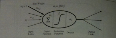
Neural networks are composed of nodes or units called neurons which are connected by directed links.
A basic neuron looks like the above image.
A link from unit `i` to unit `j` serves to propagate the activation `a_i` from `i` to `j`. (This of this as something like an electrical signal).
Each link has a numeric weight `w_(ij)` associated with it, which determines the strength and sign of the connection.
We will assume each unit has a dummy input `a_0 = 1` with an associated weight `w_(0,j)`.
To compute the output of unit j
`j` first computes a weight sum of its inputs:
`i\n_j = sum_(i=0)^n w_(i,j)a_i`.
Then, it applies an activation function `g` to this sum to derive the output:
`a_j = g(i\n_j) = g(sum_(i=0)^n w_(ij) a_i)`
This output could then be fed into several other neurons.
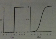
Perceptrons
The activation function `g` is typically either a hard threshold or a logistic function (see above image).
In the former case the neuron would be called a perceptron, in the later case, a
sigmoid perceptron.
Making Networks
There are two common ways to connect neurons together to make networks: make connections in only one
direction without back lines (a feed-forward network) or to allow output to go back and serve as inputs (a recurrent network).
Networks that use the latter approach can exhibit oscillatory or even chaotic behavior, so are harder to analyse (probably more realistic).
So we will focus on feed-foward networks for now.
Feed-forwards networks are usually arranged into layers such that each unit receives input from only units in the immediately preceding layer.
Layers which are not directly connected with inputs or outputs are called hidden layers.
Next day we discuss learning in such feed-forward networks.