Command, Data, and Demand Driven Paradigms

Finite State Machines

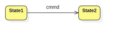
A finite state machine is a directed graph. Nodes represent states of some hypothetical computing machine, M. Arrows are labeled by commands from some hypothetical programming language L. We interpret the arrow as a state transition. For example, the following arrow means "when M executes command cmmd, M will transition from State to State2."

Command-Driven Programming

Imagine a very simple computer, M, with a 2-bit memory. The possible states are 00, 01, 10, and 11. An instruction set for M consists of two commands: inc0 and inc1. The inc0 command increments the right bit of the state by 1 modulo 2. The inc1 command increments the left bit by 1 modulo 2. Here's M's graph:

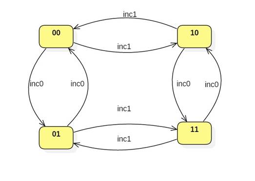
A program is a sequence of inc0 and inc1 commands. For example, starting in the state 00, the program P = {inc0; inc0; inc1} would put M in state 10.

Data-Driven Programming

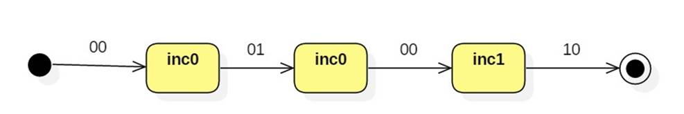
Turning things around, suppose the nodes of a directed graph represented the instructions of a program and arrows were labeled by states. In this model we think of instructions as functions that map state vectors to state vectors

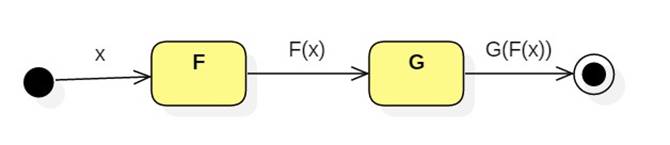
Here's our program viewed as a dataflow machine:

Dataflow is similar to functional programming.

Spreadsheets are good examples of data-driven languages.

Demand-Driven Programming

Demand-driven programming is similar to data-driven, but begins with a series of requests for data that propagate backward through the data-flow machine:

Demand-driven programming has the advantage that no unnecessary computations are done.

The concept of demand-driven programming arises in these contexts:

·       Lazy vs. eager parameter passing mechanisms.

·       Lazy vs. eager execution algorithms.

·       Thunks and delayed execution.

·       Promises.