Growth
Population dynamics looks for patterns in the ways a population changes over time. This could refer to the birth and death rates of agents or it could refer to the numbers of agents infected with a virus.
Growth and Decay
Assume rabbits in a field reproduce with a probability of r and die with a probability of d, then the population fluctuates according to the equation
population(t + delta) =
population(t) + r * population(t) – d * population(t)
= (1 + r – d) *
population(t) = c * population(t)
if r > d, then the population grows exponentially:
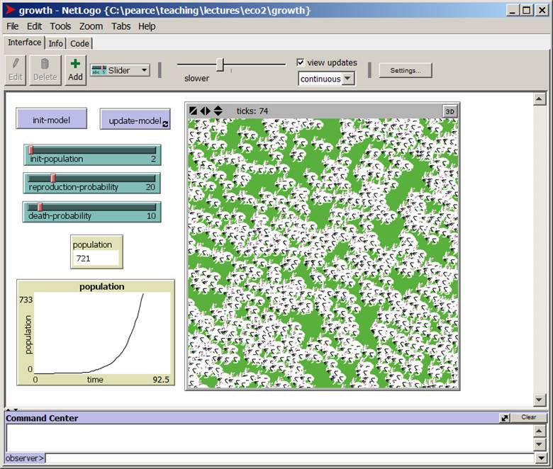
Logistical Growth
More realistically the field where our rabbits live has a carrying capacity, the largest number of rabbits the field can support. For example, rabbits eat grass, and grass grows back at a fixed rate. We would therefore expect to see the rabbit population curve to be S-shaped: initially low, followed by exponential growth, and then leveling off as the carrying capacity is reached.
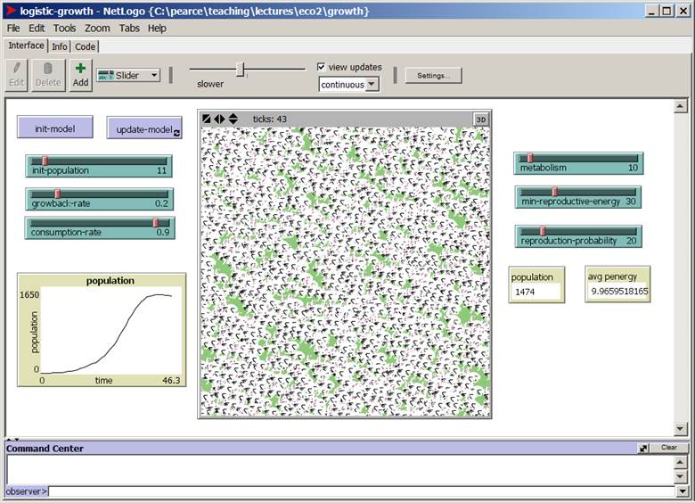
In fact, the S-curve, called logistical growth, is seen in many places: the spread of a virus, the spread of a rumor or meme, etc.
Here are a few more examples:
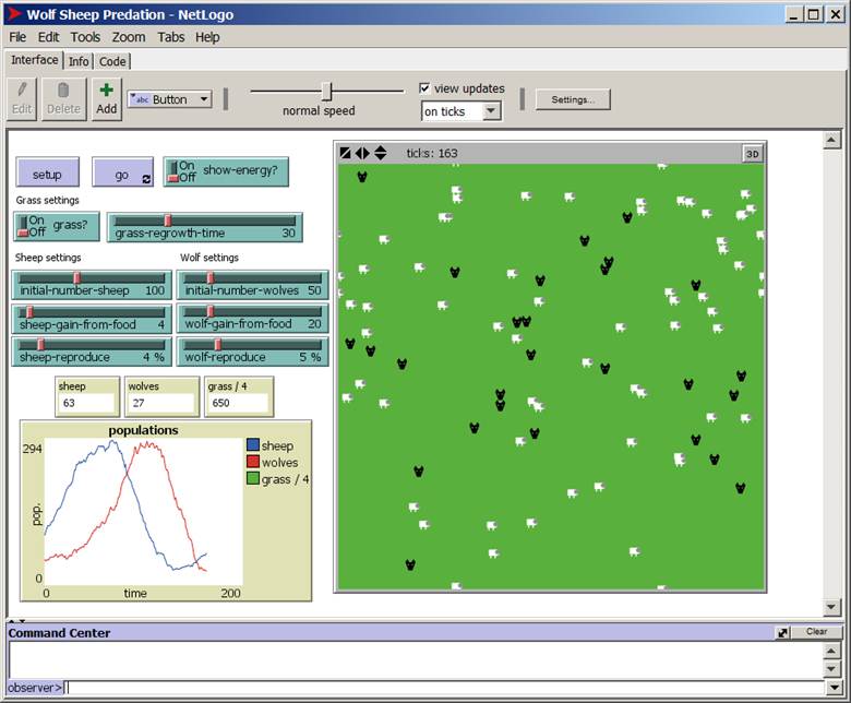
Oscillation: Predators and Prey
In a predator-prey model there are two breeds of turtles: wolves and sheep. As the sheep population rises, the wolf population rises. As the wolf population rises, the sheep population decreases. As the sheep population decreases, the wolf population decreases. As the wolf population decreases, the sheep population increases and the cycle repeats, creating a pattern of two sine waves, one behind the phase of the other: