Outline
- Online Filtering
- In-Class Exercise
- Language Categorization
Introduction
- On Monday, we started looking at how to make IR systems capable of handling longstanding recurring information needs.
- Some examples of these were (a) determining the language a document or query was written in, (b) medical news update delivery,
(c) removing spam content from email
- (a) is an example of classification: assigning a label to a document.
- (b) is an example of filtering: sending documents to different locations based on who has what information need.
- We begin today by looking at (b) in more detail...
Topic-Oriented Batch Filtering
- Consider the health-care task we presented earlier.
- At the start, there are no documents. As new documents arrive, we could imagine filtering them.
- If we can afford to wait, we can accumulate documents into a corpus, index them, apply a search technique like BM25 to rank them according to the health categories desired, and send them to the appropriate users.
- We can then wait for more documents to arrive and repeat the process.
- This approach is called batch filtering.
- This approach is viable if enough documents arrive within the repetition window, say once a week, once a month, etc.
Example of Topic Oriented Filtering
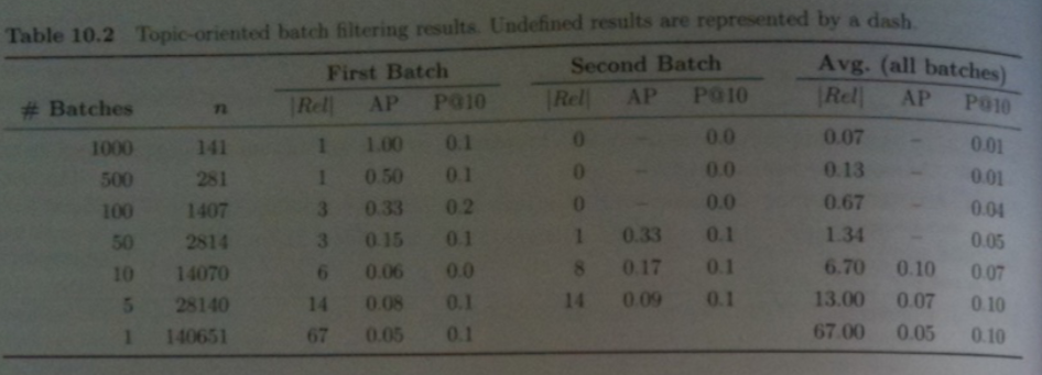
- The above table shows the results of doing batch filtering for our medical task (Topic 283) on the TREC 45 corpus using BM25.
- The query used to rank documents for relevance was `langle` "mental", "illness", "drugs" `rangle`.
- `N=140,651` Financial Times articles from 1993 onward in TREC45 were used. Of these 67 were relevant to Topic 283.
- Four character char grams were used for tokens. (According to the book, stemming and not stemming approaches yielded similar results).
- Documents were grouped into batches of fixed size, depending on the experiment. For example for the 1000 batch experiment, the batch size consisted of 141 documents.
- Each batch was indexed independently of the rest of the collection. Each batch is presented to the BM25 filter one at a time in chronological order.
- To evaluate the results of more than one batch, the table above shows the simplistic approach of evaluating each performance measure separately for each batch, then average these results to compute a summary measure.
Issues With Evaluating the Result
- Some problems with evaluating as we did on the last slide are:
- When we divide into more batches, the number of documents/batch goes down, and so the likelihood a batch has no relevant documents increases. (`|Rel| = 0`). `AP` (average precision) will be undefined if any batch has `|Rel|=0`. So any measure that depends on `|Rel|` will not work for small batches.
- Measures like precision at `k` are heavily influenced by `n`, making it impossible to compare results from different batch sizes.
- We can see these effect in our tables from the last slide -- the `AP` values for the Second Batch as well as the average are undefined for greater than 10 batches. Both the `AP` and `P`@`10` results also don't seem to be very stable with respect to batch size.
Size-Specific Precision at `k`
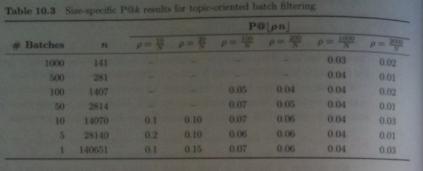
- One way to solve the issue with `P`@`k` of the last slides is to compute size specific `P`@`k`. I.e., `k` used for evaluating batches sizes of size `n` is set to `\lfloor rho n\rfloor` where `rho` is some constant.
- Typically, `rho` is chosen to be `k/N` where `N` is the corpus size and `k` is roughly the total number of documents presented to the user.
- The table above show using this approaches gives more stable results across batch sizes.
Aggregate Precision at `k`
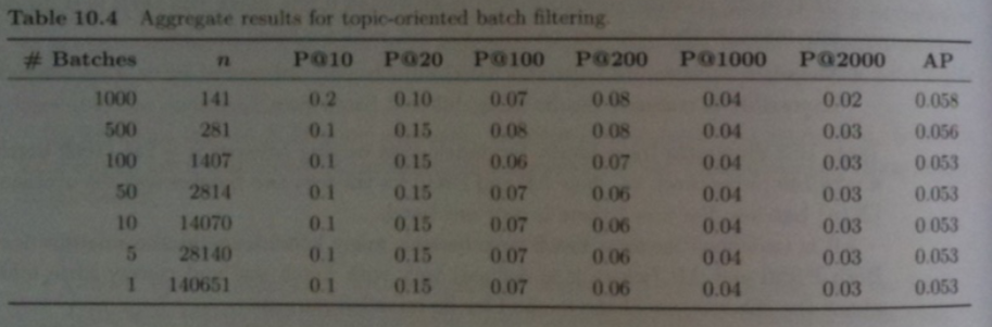
- One drawback with size specific precision at `k`, `P`@`k`, is that the number of relevant documents can vary between batches, but we are always using the same value for `k`.
- Instead, of fixing `k` across all of our batches of a given size, we can use the fact that we have a scoring function `s` (BM25 in our example) and in a given batch present to the user all documents which have a relevance score above some threshold `t`.
- We choose `t` so that `k=rho N` documents will have score `s >t`.
- We define aggregate `P`@`k` and `AP` using this thresholding idea.
- The table above shows this approach is even more stable than Size-Specific Precision and AP.
In-Class Exercise
- Give a concrete procedure for computing aggregate P@100 if our corpus has `N=1000` documents where the batch size is `100`.
- Assume `X` documents in the corpus have a scoring function score over `N-X`.
- Please post your solution to the May 12 In-Class Exercise Thread.
Online Filtering
- Online filtering is essentially batch filtering where the batch size is 1.
- An online filter must act immediately on each message in a sequences rather than on batches of messages.
- Messages deemed relevant must be delivered and all others discarded.
- Delivery might be an email to an inbox or text message or sending a message to some folder.
- If possible we would like to be able to flag messages by priority. I.e., have some kind of primitive importance ranking.That way we don't need to discard messages.
- Otherwise, we need to set some relevance threshold so that the rate of delivery `rho` represents a good balance of precision and recall as measure by a score like an F-measure.
- Scores like BM25 when used to give a priority score need to be modified so they can work on a per-document basis. For example `N_t` assumes a large collection of documents. To fake this one can just assume the corpus consists of the single current document.
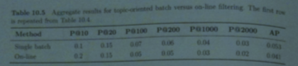
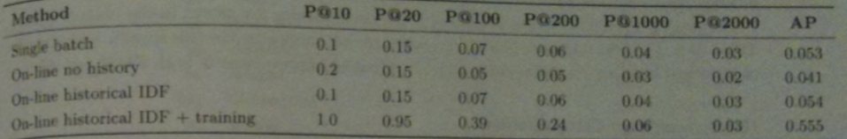
- Above shows the aggregate precision scores for online filtering using BM25 and a theshold that gives a given target (10, 20, 100, etc) number of results over the whole collection versus single batch filtering (whole corpus 1 batch).
Historical Collection Statistics
- At the time we deploy a filtering system we might not know the rate at which relevant documents arrive, making it harder to choose thresholds, etc.
- We next consider how to take advantage of this kind of information.
- If we are doing batch filtering, one way to take advantage of historical information.
- In the batch setting, we can do this by historical documents with a given batch to do ranking, then removing the historical documents leaving a rank and score for the documents in the batch.
- This will mean the batch makes use of better collection statistics such as IDF scores and so the relevancy scores determined will be more accurate.
- Rather than return a fixed number of documents per batch, we can return only those documents that appear in the top `k' > k` in the combined list
- For a suitable `k'` this will return the same number of documents overall while achieving better precision.
Online Filtering with Historical Collection Statistics -- What to Store
- When historical documents are used online filtering effectively reduces to batch filtering.
- One difference is that we only need to figure out where a single documents score is relative the list we have already computed.
- Hence, we don't need to build a full inverted index apparatus we have previously considered.
- All we need to compute BM25 or a similar score is a dictionary with entries indicating `N_t` for each term. For overall ranking, we might also keep an ordered list of historical scores (with respect to all terms, not per term scores).
- We can compute relevance using the current document and `N_t`. To compute rank we binary search in the list to insert the score of the current document.
- The table above compares online filtering with and without use of historical information.
- We haven't explained the last row of the above table yet.
Historical Training Examples
- In the filtering setting it is likely that some examples of relevant documents are already known.
- For example, before we start filtering medical papers related to cardiac surgery, we probably have some known examples of papers on this subject.
- Such examples are known as training examples or labeled data.
- In machine learning, building a classifier using labeled data is known as supervised learning.
- Using BM25 relevance feedback is an example of how we could build such a classifier.
- I.e., we could look at the `r` known relevant documents, select the top `m` term scores with respect to these documents, say `m=20` and then augment our original query with these terms.
- This was used to produce the last row of results from the previous slide for the query we had last day using TREC45 data.
Language Categorization - Filtering
- Two common tasks associated with documents and the language they are written in are:
- Categorization: Given a document `d` and a set of possible categories, identify the category to which `d` belongs. Related to this is Category Ranking: rank the category according to how likely the document belongs to that category.
- Filtering: Given a category `c` determine which documents belong to this category. Related to this is document ranking list the documents in order of the likelihood of belong to the category.
- The book's authors used the random link feature of Wikipedia to collect 8012 articles from each of 60 languages from Wikipedia.
- They then extracted the first 50 bytes of text from each article as snippet messages.
- They used 4000 snippets for training and 4012 for categorization and filtering.
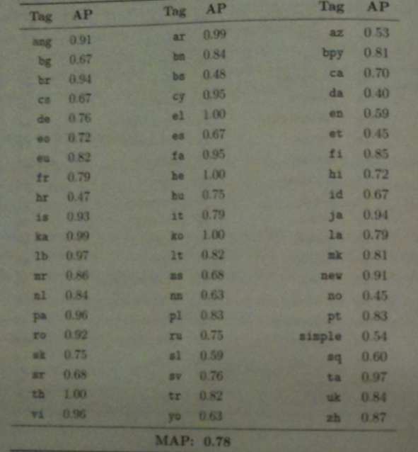
- To do filtering, each language was treated as a separate topic. Snippets were 4-grammed and training snippets grams were used as query terms in BM25 document ranking for test documents. (I.e., from the 4000 snippets take all in a given language and thenall 4-grams thereof - treat that as the query for BM25 ranking).
- The graph above shows the results of this document ranking experiment.
Language Categorization - Categorization
- To perform categorization we have to rank languages instead of documents.
- To do this we use the relevance scores from the document ranking.
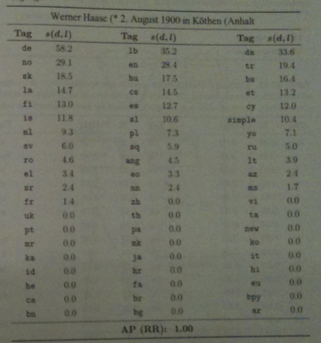
- Given a document `d` and a language `l`, let `s(d,l)` be the relevance score for `d` in the document ranking for `l`.
- Given two language `l_1` and `l_2` we assume if `s(d,l_1) > s(d,l_2)` that `d` is more likely to be written in `l_1` than `l_2`.
- The table above shows the complete ordering of BM25 scores for each language for a snippet of German text.
- In this setting P@1 is most commonly called accuracy. This indicates the proportion of documents for which the correct category was ranked first.
- MAP scores in this setting are equal to Mean Reciprocal Rank (MRR) scores because there is exactly one relevant result per ranking.
- For a single topic, reciprocal rank is defined as `\R\R=1/r` where `r` is the rank of the first and only relevant result. In the case `AP = P`@`r =1/r`.
- Summary statistics are often expressed as either micro-averages which are computed over all documents without regard to category or macro-averages which are an average of summary measures computed for each category.
- For the accuracy and the language categorization tests just considered both of these scores were 0.79. For MRR, the scores were 0.860 and 0.857 respectively.
div class="slide">
On-line Adaptive Spam Filtering
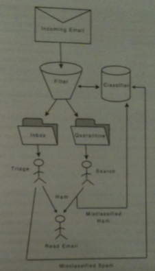
- The above figure illustrates the flow of an incoming email through a spam filter.
- Emails arrive one-by-one (i.e., the system is online).
- If an email is labeled as spam in goes into a quarantine folder. It may be rescued from this folder and read or not.
- On the other hand, a user might label mail that the filter said was okay (ham, and hence put in the Inbox) as spam.
- Such relabeling's are used provided as examples to the classifier which then improves itself for subsequent mail (i.e., the system is adaptive).
- For our example, we will consider the inbox to be a queue and the quarantine a priority queue with the hardest to classify ranked at the top of the queue.
Framework for Categorization
- One tool for evaluating spam filtering is the TREC 2005 Public Spam Corpus.
- This consists of a sequence of 92,180 messages, of which 39,399 are spam and 78,798 are ham.
- Rather than splitting the sequence into training and tests sets, on-line feedback is used.
- In this setting, an ideal user is assumed to detect and report all errors.
- So every message may be used as a historical training example immediately after it is delivered.
- The online scenario is implemented using the TREC Spam Filter Evaluation Toolkit.
- This toolkit can be used for any binary classification task (we have two exclusive categories), although we are using it for just spam versus ham.
- For evaluation, within the toolkit's framework, a filter must support following operations:
- initialize - Create a filter a process a new stream of messages
- classify file - Return a category and priority for the message in file.
- train spam file - Use file as a historical example of spam.
- train ham file - Use file as a historical example of ham.
- finalize - shutdown the filter.
BM25 Applied to On-line Adaptive Email Filtering
- We now give an example of using this framework together with BM25 for Spam filtering.
- To start we call initialize to create an initial filter which has no information on which to base its decision.
- The rate and manner in which this filter improves with training is known as the learning curve.
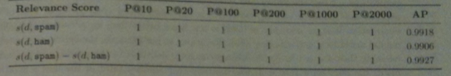
- We apply BM25 with relevance feedback separately to each of the document ranking problems: identifying spam and identifying ham.
- This yields two scores: `s(d, spam)` and `s(d, ham)`.
- The category ranking for `d` is determined by the difference `s(d) = s(d,spam) - s(d, ham)`.
- If `s(d) > 0` the document is classified as spam, otherwise, it is classified as ham.
BM25 Applied to Adaptive Email Filtering -cont'd
- In their experiments, when either a train ham or train spam is called, the book's author's filter generates 4-grams from the message and keeps track of the average length of the spam or ham document and `N_t` for that term.
- When classify file is called, a BM25 score is computed with respect to the 4-grams in file and these `N_t` and average length values for both spam and for ham. Finally, `s(d)` is calculated.
Evaluation
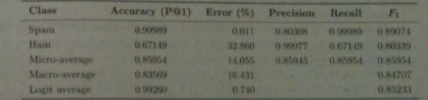
- The above shows the evaluation measures for the primary categorization problem in an on-line spam filter.
- For `F_1` score we assume spam constitutes the relevant class is spam
- Notice the P@1 score for spam is very high.
- Instead, error `1-P`@`1` expressed as a percentage is often used.
- So an error rate of .1% is 10 time better than one of 1%.
- The above shows that about 1 in 10000 spam messages is delivered to the user's in-box.
- On the other hand, the ham error rate is 32.9% so about a third of good messages are quarantined.
- This is probably unacceptable, but the reverse situation might not be.
- Micro-average and macro-average scores fail to take into consideration the prelavance of spam. So doubling the amount of ham while keeping the amount of spam the same actual would improve both error rates.
- To compensate for this, we can use a logit average LAM. Here `LAM(x,y) = logit^{-1}((logit(x) +logit(y))/2)` is often used.
Choosing a threshold
- Rather than accept the ham error rate above the book explores setting different values for `t` and then considering `s(d) > t` as spam
.
- For example, when `t=2156` the spam error is 56.8% but the ham error rate is 0%. On the other hand, when `t=-180` the spam rate is 0 and the ham rate is 34.9%.
- One can use this to choose the best compromise that the filter offers for the two errors.
- We can also plot the points (spam error, ham error) for fixed `t` as we let `t` vary. This gives the so-called receiver operating characteristic (ROC) curve.
- To compare filters one often looks at 1-AUC (area over this curve) expressed as a percentage.
- The book shows the score for this filter versus spam assassin are comparable.


