Outline
- Introduction to Linear Algebra
- In-Class Exercise
- Perceptons
Introduction
- Last week and Monday, we began talking about machine learning.
- We introduced a little about probability theory, then talked about the Probably Approximately Correct (PAC) definition of learning.
- I said we were going to give an example class that is PAC-learnable by perceptrons. Before doing this, though, we needed to review a little linear algebra and define perceptrons, our first machine model of a neuron.
- So we covered scalars, vector, and matrices as mathematical objects.
- We defined linear dependence, independence, and space. We defined the notion of vector space.
- Before introducing perceptrons, we finish up this review today by looking at matrix operations, orthogonality, determinants, matrix inverses, and some special kinds of matrices.
Matrix Operations
- We call a matrix with all its coordinates `0` the zero matrix, `mathbf{0}`; we call a vector with all its coordinates `0` the zero vector, `mathbf{0}`.
- Given a matrix `M` or a vector `vec{v}`, we can multiply it by a scalar `c`. The coordinates of the result are given by `(c \cdot M)_{i,j} = c cdot M_{i,j}` and `(c \vec{v})_i = c \cdot \vec{v}_i`. For example,
`3 \cdot [[1, 2], [3, 4]] = [[3, 6], [9, 12]]` and `2 cdot [[1],[-1]] = [[2],[-2]]`.
- Given two matrices `A`, `B` or vectors `vec{v}`, `vec{w}` we can also add them. The coordinates of the result are given by `(A + B)_{i,j} = A_{i,j} + B_{i,j}` and `(v + w)_i = v_i + w_i`. For example, `[[1],[-1]] + [[2],[2]] = [[3],[1]]`.
- We note matrices have an additive inverse as `M + (-1)M = mathbf{0}`.
- We will call any of the above operations a linear combination. Given a set `vec{x}_1, vec{x}_2, ..., ` of vectors `X`, we call the set of all vectors that can be created by
taking linear combinations of these vector the span of `X`, denoted `span(X)`.
- If an equation `vec{v} = \sum_{i=1}^m a_i vec{w}_i` holds, then we say `vec{v}` is linear dependent on `vec{w}_1, ..., vec{w}_n`. If no scalars `a_i` exists such that an equation of this type holds, then we say `vec{v}` is linearly independent of `vec{w}_1, ..., vec{w}_n`.
- We'll call a subset `V` of `\mathbb{F}^n` containing `mathbf{0}`, closed under addition and multiplication by scalars, a vector space.
More Matrix Operations
- Given an `A in \mathbb{F}^{m times n}` we can create a matrix, `A^{\top}`, where we swap `A`'s rows and columns: `(A^{\top})_{i,j} = A_{j,i}`. For example,
`[[1, 2], [3, 4], [5, 6]]^T = [[1, 3, 5],[2, 4, 6]].`
- Given `A in mathbb{F}^{m times n}` and `B in mathbb{F}^{n times p}`, we can define their matrix product `C=AB` as `C_{i,j} = sum_k A_{i,k}B_{k,j}`. For example,
`[[1, 2], [3, 4], [5, 7]] [[1, 1], [-1, 0]] = [[-1, 1], [-1, 3], [-2, 5]]`.
- Matrix multiplication is associative, `A(BC) = (AB) C`, and distributes over "`+`", `A(B+C) = AB +AC`, but it is not generally commutative. That is, often `AB ne BA`. For example, `[[-1,1],[1,0]] = [[1,-1],[0,1]] [[0,1],[1,0]] ne [[0,1],[1,0]] [[1,-1],[0,1]] = [[0,1],[1,-1]]`.
- Given two `n`-dimensional vectors `vec{v}`, `vec{w}`, we can view them as matrices and multiply them as, `vec{v}^{top}vec{w}`. This is called the inner product of `vec{v}`, `vec{w}` and will be a `1 times 1` matrix, that we'll view as a scalar. (When `mathbb{F} = CC`, you need to take the complex conjugate of the components of `vec{v}` for this to make sense.)
- We can check/prove-by-induction `(AB)^{\top} = B^{\top}A^{\top}`, and so `vec{v}^{top}vec{w} = vec{w}^{top}vec{v}`.
- In high school, we are often asked to solve systems of linear equations such as:
`2x+4y = 7`
`-3x + 2y = 20`
we can always write as a matrix equation. For example,
`[[2, 4],[-3, 2]][[x],[y]] = [[7],[20]]`.
The general format of this equation is `A vec{x} = vec{b}`.
Norms
- Taking the inner product of a vector with itself gives `vec{v}^{top}vec{v} = sum_i (v_i)^2`. Taking the square root of this, geometrically represents the standard euclidean distance of `vec{v}` from the origin. We write this as `||vec{v}|| = (vec{v}^{top}vec{v})^{1/2}`. This is called the norm of `vec{v}`. Sometimes we will also write this as `||vec{v}||_2` when we want to emphasize it is the `L_2` norm. In general, the `L_p` norm of `vec{x}` is defined as `||x||_p = (sum_i |x_i|^p)^{1/p}`.
- Given two vector `vec{x}` and `vec{y}`, one can verify that `||vec{x} - \vec{y}||` satisfies the definition of a metric, and so we can use this in the definition of PAC learning.
- One can also prove that `vec{v}^{top}vec{w} = ||vec{v}^{\top}|| ||vec{w}|| cos theta`, where `theta` is the angle between the two vectors, so the inner product has a geometric interpretation.
- We will finish up our discussion of linear algebra next day.
Normalization, Orthogonality
- Recall for `\vec{u}, \vec{v} in mathbb{F}^n`, we defined the inner product as `(\vec{u} , \vec{v}) = \vec{u}^{top}\vec{v} = sum_{i=1}^n u_iv_i` and defined the norm as `||u|| = (\vec{u} \cdot \vec{u})^{1/2}`. If the field is `CC`, we should take the complex conjugate as well as the transpose of `\vec{u}` in our defintion.
We sometimes also write inner product as `\vec{u} cdot \vec{v}` rather than `(\vec{u} , \vec{v})`.
- Geometrically, we said `\vec{u} \cdot \vec{v} = ||\vec{u}||||\vec{v}|| cos theta`, where `theta` is the angle between these vectors.
- Given a vector `vec{v}`, the vector `hat{v} := vec{v}/{||vec{v}||}` is a vector of length 1 (I.e., `||hat{v}|| = 1`) which points in the same direction as `vec{v}`.
- We call a vector of length 1, a unit vector. We will tend to use a hat rather than an arrow above a vector to indicate it is a unit vector.
- The process of creating a unit vector from a vector as above is called normalization. For example, we can normalize `[[1],[1]]` as `[[1/sqrt(2)], [1/sqrt(2)]]`.
- We say two vectors are orthogonal if `\vec{u} \cdot \vec{v} = 0`. If `\vec{u} ne mathbf{0}` and `\vec{v} ne mathbf{0}`, this implies `theta` is either `\pm pi/2`, so they are perpendicular. For example, `[[1],[1]]` and `[[1],[-1]]` are orthogonal, but `[[1],[1]]` and `[[1],[0]]` are not.
- If `\vec{u}, \vec{v}` are orthogonal and unit vectors, we say they are orthonormal.
Bases
- Recall if an equation `vec{v} = \sum_{i=1}^m a_i vec{w}_i` holds, then we say `vec{v}` is linear dependent on or `vec{v}` is in the span of `vec{w}_1, ..., vec{w}_n`. If no scalars `a_i` exists such that an equation of this type holds, then we say `vec{v}` is linearly independent of `vec{w}_1, ..., vec{w}_n`.
- For example, `[[1],[0]] = [[1],[1]] + [[1],[-1]]`, so `[[1],[0]]` is linearly dependent on `[[1],[1]]` and `[[1],[-1]]`.
- Recall also we said a subset `V` of `\mathbb{F}^n` containing `mathbf{0}`, closed under vector addition and multiplication by scalars, is a vector space. (You can give a more general definition than this. Remember we are using `mathbb{F}` to mean some field such as `RR`, `CC` or `ZZ_n`.)
- A set of linearly independent vectors which span `V` is called a basis for `V`.
- Notice a set of orthogonal vectors `X` will be linearly independent.
- A set of orthonormal vectors `X` which span `V` is called an orthonormal basis.
- For example, `\{\ [[1],[0]], [[0],[2]]\}` is a basis for `\mathbb{R}^2`, `\{\ [[1/sqrt(2)],[1/sqrt(2)]], [[1/sqrt(2)],[-1/sqrt(2)]]\}` is an orthonormal basis `\mathbb{R}^2`.
Dual Spaces, Tensors
- Given a vector space `V` over `mathbb{F}`, a linear functional is a map `f:V -> \mathbb{F}`, such that for any vectors `vec{u}, vec{v} in V` and `a,b in \mathbb{F}` we have `f(a\cdot vec{u} + b\cdot vec{v}) = a \cdot f(vec{u}) + b \cdot f(vec{v})`.
- Given two linear functionals `f`, `g` and a scalar `b`, we can define `(b\cdot f)(vec{u})` as `f(b\vec{u})` and `(f + g)(vec{u})` as `f(vec{u}) + g(vec{u})`.
- The space of linear functionals on `V` closed under these operations is called the dual space of `V`, and is denoted `V^\star`.
- Notice for any vector `vec{w}` that `vec{w}^{\top}(a\cdot vec{u} + b\cdot vec{v}) = a \cdot vec{w}^{\top}vec{u} + b \cdot vec{w}^{\top}vec{v}`, so `vec{w}^{\top}` can be viewed as a linear functional.
- It turns out that given a basis `u_1, ..., u_k` for `V \subseteq mathbb{F}^n` (let's assume things are finite dimensional), then `u_1^{\top}, ..., u_k^{\top}` will be a basis for `V^\star`.
- Notice the inner product also satisfies `(a cdot vec{u}+ b cdot vec{v}, vec{w}) = a(vec{u}, vec{w}) + b(vec{v}, vec{w})`. Our previous discussion showed in was linear in its second argument. So it is linear in both argument.
- An operation that takes `k` many vectors, is linear in each input, and produces an element of `\mathbb{F}^m` for some integer `m \geq 1` is called a multilinear map or tensor. So inner product is a 2-linear (bilinear) map.
- We will use tensors to say how different layers in a neural net are connected.
Identity and Inverse Matrices
- The `n times n` matrix `I` with 1's along the diagonal, and 0's elsewhere is called an identity matrix.
- Given any `n times n` matrix, `A`, one can verify that `A = AI = IA`.
- We say a `n times n` matrix `A^{-1}` is the inverse of `A` if `A^{-1}A = I`. For example,
the inverse of `[[1,1],[1,-1]]` is `[[1/2,1/2],[1/2,-1/2]]`.
- Not all matrices have inverses. For example, `[[1,0],[0,0]]` does not have an inverse.
- We can solve a linear equation `A\vec{x} = vec{b}` for `vec{x}`, if an inverse exists, as `\vec{x} = A^{-1}vec{b}`.
- One way to compute the inverse of a matrix `A`, if it exists, is to write the matrix `[A|I]` then use row operations (add scalar multiples on one row to another), to convert this, step-by-step to a matrix`[I|A^{-1}]`.
- We now restrict our attention to real matrices. An `n times n` matrix all of whose rows are orthonormal and all of whose columns are orthonormal is called an orthogonal matrix. For orthogonal matrices, `A` we have `A A^{top} = A^{top}A = I`
Determinants
- Given an `n times n` matrix `A`, its determinant, `|A|`, is the value of the unique multilinear map (viewing `A` as `n` row vectors of size `n`) with range `\mathbb{F}`, which is 1 on the identity matrix and 0 if two rows are the same.
- Multilinearity in rows and the identity matrix having determinant 1, let's us immediately compute the determinant of a diagonal matrix, a matrix with nonzero entries only along the diagonal. For example, `|[[a_1, 0],[0, a_2]]| = a_1 |[[1, 0],[0, a_2]]| = a_1\cdot a_2 |[[1, 0],[0, 1]]| = a_1\cdot a_2 cdot 1 = a_1\cdot a_2`.
- Let `A[j,i]` be the matrix with all the same entries `A` except that the `j`th row has the same entries as `A`'s `i`th row. Let `R_i` be the `i`th row of `A`. So `|A[j,i]| = 0` as it has repeated rows, and `|[[R_1],[...],[R_{j-1}],[R_j + c\cdot R_i],[R_{j+1}],[...],[R_n]]| = |A| + c|A[j,i]| = |A|`, by multilinearity.
- This shows we can add a scalar multiple of one row to another without changing the determinant.
- Using the above property, we can convert any matrix `A` to an upper triangular matrix, a matrix with nonzero entries only on or above the diagonal, with the same determinant. We can convert an upper triangular matrix to a diagonal one by more row operations without affecting the diagonal, so once we get an upper triangular matrix, we can take the product of its diagonal entries to get the determinant.
Determinants Properties
- The determinant is also column multi-linear. (Is implied by row using multi-linearity).
- Swapping two rows of `A` or swapping two columns of `A` yields a sign change in the determinant. (Is implied by using multi-linearity).
- `|AB| = |A||B|`. (To see this let `A_i` denote the `i`th row of `A`, verify `(AB)_i = A_iB`, then verify `|[[A_1B],[...],[A_nB]]| = |A||B|`.)
- (3) above implies, if `|A|` is 0, then the matrix can't be inverted.
- Let `n ge 2`. Given an `n times n` square matrix `A`, the `k,j` minor `A_{kj}` is the `n-1 times n-2` square matrix obtained by deleting the `k`th row and `j` column. Given
this definition, using column multi-linearity and (2) abbove, one can show: `|A| = sum_{j=1}^n(-1)^{k+j}a_{kj}|A_{kj}|.`
- Using (5), and induction, one can show `|A|` equals the area/volume/hypervolume of the parallogram/parallelpiped/parallelotope determined by the rows of `A`.
Lines, Planes, Hyperplanes
- The dimension of a vector space `V` is the number of elements in any basis for it.
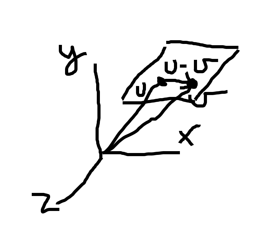
- For `n> 3`, if `V` is an `n`-dimensional vector space, a set `P subseteq V` is called a hyperplane if the set of difference vectors `vec{p_1} - vec{p_2}` for `vec{p_1}, vec{p_2} in P` form an `n-1` dimensional vector space. When `n=3`, it is called a plane, when `n=2` it is called a line. Since `V` is `n`-dimensional such a vector exists.
- We call a vector which is orthogonal to the `n-1` dimensional vector space in `V` a normal to the hyperplane/plane/line.
- The image above show the `n=3` case. Here `vec{x}` and `vec{p}` are two points on the plane. Their difference is a tangent in the plane.
In the above `vec{n}` is the normal.
- A point `vec{p}`, a normal `vec{n}` fully determine a hyperplane as those points `vec{x}` which satisfy: `vec{n}(vec{x} - vec{p}) = 0`.
- Often it is useful to use a unit normal `hat{n} = vec{n}/||vec{n}||` rather than an arbitrary normal when talking about planes and arbitrary points `vec{x}'` so that length components of `vec{x}'` out of the plane is preserved (not stretched).
- Given an arbitrary point `vec{x}'`, not necessarily on the plane, we can compute its distance to the plane, as `||hat{n} cdot (vec{x}' - vec{p})|| = ||vec{n}||^{-1}||vec{n} cdot(vec{x}' - vec{p})||`.
Other Hyperplane Equations, Halfspaces
- Let `d = vec{n} cdot vec{p}`. Then sometimes our hyperplane equation is a rewritten as `vec{n} cdot vec{x} = d`.
- In the case. of a plane, if we take the normal to be the vector `[a, b, c]^T`, and `vec{x} = [x, y, z]^T`, this gives the familiar high school equation for a plane:
`ax + by + cz = d`.
- We call the set of points satisfying an inequality like `vec{n} cdot vec{x} ge b`, a halfspace.
Perceptrons
- Let's return from linear algebra now to neural networks.
- The basic unit of our neural nets will be some kind of artificial neuron whose definition is often motivated from biology.
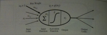
- Rosenblatt's neuron (1959) looks like the above image. The image imagines that a neuron receives several inputs and may be connected to several outputs.
- A link from neuron `i` to neuron `j` serves to propagate the activation `a_i` from `i` to `j`. (Think of this as something like an electrical signal).
- Each link has a numeric weight `w_(ij)` associated with it, which determines the strength and sign of the connection.
- To compute the output of unit j
- `j` first computes a weighted sum of its inputs:
`i\n_j = sum_(i=1)^n w_(i,j)a_i`.
- Then, it applies an activation function `g` to this sum to derive the output:
`a_j = g(i\n_j) = g(sum_(i=1)^n w_(ij) a_i)`.
- The above set-up let's us define essentially a whole layer of perceptrons. If we want, just one perceptron (one output), we can simplify this to `a_{out} = g(i\n) = g(sum_(i=1)^n w_(i) a_i)`.
Choice of Activation Function
- Let `theta in RR`.
- There are several possible choices one could have for the activation function:
- We can choose `g` to be a step function at `theta`, i. e., it has value `0` when `x < theta` and `1` otherwise. This is useful if we want the output function to be boolean valued.
- We can choose `g` to be the logistic function `1/(1 + e^{-(x - theta )}) = 1/2 + 1/2tanh((x - theta)/2)`. This is function is differentiable. As `x` gets much smaller than `theta` this is equal to 0, and as `x` gets much bigger than `theta` is equal to 1. The differentiability is a useful property for gradient descent based methods to compute neuron weights.
- We can choose `g` to be a rectified linear unit (relu), `max(0, x - theta)`. This function is continuous everywhere and it is differentiable everywhere but at `theta`. For many gradient descent algorithms this turns out to be sufficient and to work better in practice.
Perceptron Update Rule
- Suppose we want to train a perceptron to output `1` when given a boolean vector `vec{x}` in some `X subset {0,1}^n` and `0` otherwise.
- Here we call `X` the concept we are trying to learn.
- We could imagine starting with our weights all set to `0`. I.e., `\vec{w} = (0, ...)` and our threshold `theta = 0`.
- When we receive an example `\vec{x}`, we predict whether it is in `X` according to whether `vec{w} \cdot vec{x} ge theta`. So we are using the step function at `theta` as our activation function.
- The perceptron update rule says:
- On a correct prediction, do nothing.
- On a false positive prediction, set `vec{w} := vec{w} - vec{x}` and set `theta := theta + 1`.
- On a false negative prediction, set `vec{w} := vec{w} + vec{x}` and set `theta := theta - 1`.
Winnow
- Winnow is an alternative update rule for training perceptrons due to Littlestone 1988.
- Let `\vec{w^I}` be an initial vector of all positive weights and let `alpha > 1`. Assume `theta > 0`.
- Then on an example `vec{x}`, the Winnow update rule says:
- On a correct prediction, do nothing.
- On a false positive prediction, for all `i`, set `w_i := alpha^{-x_i}w_i`.
- On a false negative prediction, for all `i`, set `w_i := alpha^{x_i}w_i`.
- Notice the learning parameters `alpha` and `theta` for Winnow don't change once they're initially set, and the choice of their value is made by the coder on what seems to work best. These kind of "magic" constants are known as hyperparameters.
- Given the set-up on initial weights and `alpha`, at any training step using Winnow, the weights will always be positive. This limits Winnow to learn things computable by positive threshold functions unless some kind of pre-transformation is done to the inputs.
- On Wednesday, we will consider the PAC learning properties of these update rules, and start talking about Python.


