Outline
- Finish Computer Vision
- In-Class Exercise
- Speech Recognition
- Natural Language Processing
Introduction
- On Monday, we started talking about neural net applications.
- We first described hardware and techniques that might be needed for large scale NN applications such as: GPUs, distributed algorithms, etc.
- We then began talking about Computer Vision and some of the tasks it encompasses: Recognizing faces, object detection, recognition, and annotation, transcribing symbols from images, pixel labeling, image denoising, etc.
- We said that before feeding a computer vision task to a neural net, we might do some preprocessing on images such as to make all the pixel values come from a common scale, cropping or resizing images, etc.
- The goal of preprocessing is to eliminate sources of variation in our inputs which are unimportant to the learning task at hand. This usually means we can train with less data (we don't have to learn what's unimportant.)
- Today, we start by considering another kind of image preprocessing known as constrast normalization.
Image Contrast
- Contrast refers to the magnitude of the difference between bright and dark pixels in an image.
- This can be measured as the standard deviation of the pixels in an image or region of an image.
- We can imagine a image as a tensor `mathbf{X} in RR^{r times c times 3}` (`r` rows, `c` columns, red, green, blue color values). So `X_{i,j, 1}` would be the red value of the `(i, j)`th pixel. (2 - for blue, 3 - for green).
- The contrast of the entire image is then defined to be:
`sqrt(1/{3rc}sum_{i=1}^{r}sum_{j=1}^{c}sum_{k=1}^{3}(X_{i,j,k} - mathbf{bar{X}})^2)`
where
`mathbf{bar{X}} = 1/{3rc}sum_{i=1}^{r}sum_{j=1}^{c}sum_{k=1}^{3}X_{i,j,k}`
In-Class Exercise
- Imagine you have two 3x3x3 RGB images: One consisting of one red row, one blue row, and one green row, the other having all pixels red except the bottom right one which is blue.
- In each case, work out the contrast of the entire image.
- Post your solutions to the Dec 6. In-Class Exercise Thread.
Global Contrast Normalization
- As we don't usually classify based on the amount of contrast in an image, we can normalize all the images to have the same constrast.
- To do this we could divide each pixel coordinate by the image contrast. We then multiply by a fixed constant `s` so that all images have contrast `s`.
- To prevent divide by zero errors for images with no contrast (say solid color images), we add a `epsilon` hyperparameter.
- In doing this division, we also don't want to amplify the contrast of low contrast, noisy images, so we also add a `lambda` hyperparamter as part of the image contrast calculation.
- Thus, we arrive at the following formula for Global Contrast Normalization (GCN):
`X'_{i,j,k} = s(X_{i,j,k} - mathbf{bar{X}})/(max\{epsilon, sqrt(lambda + 1/{3rc}sum_{i=1}^{r}sum_{j=1}^{c}sum_{k=1}^{3}(X_{i,j,k} - mathbf{bar{X}})^2)\})`.
Local Contrast Normalization
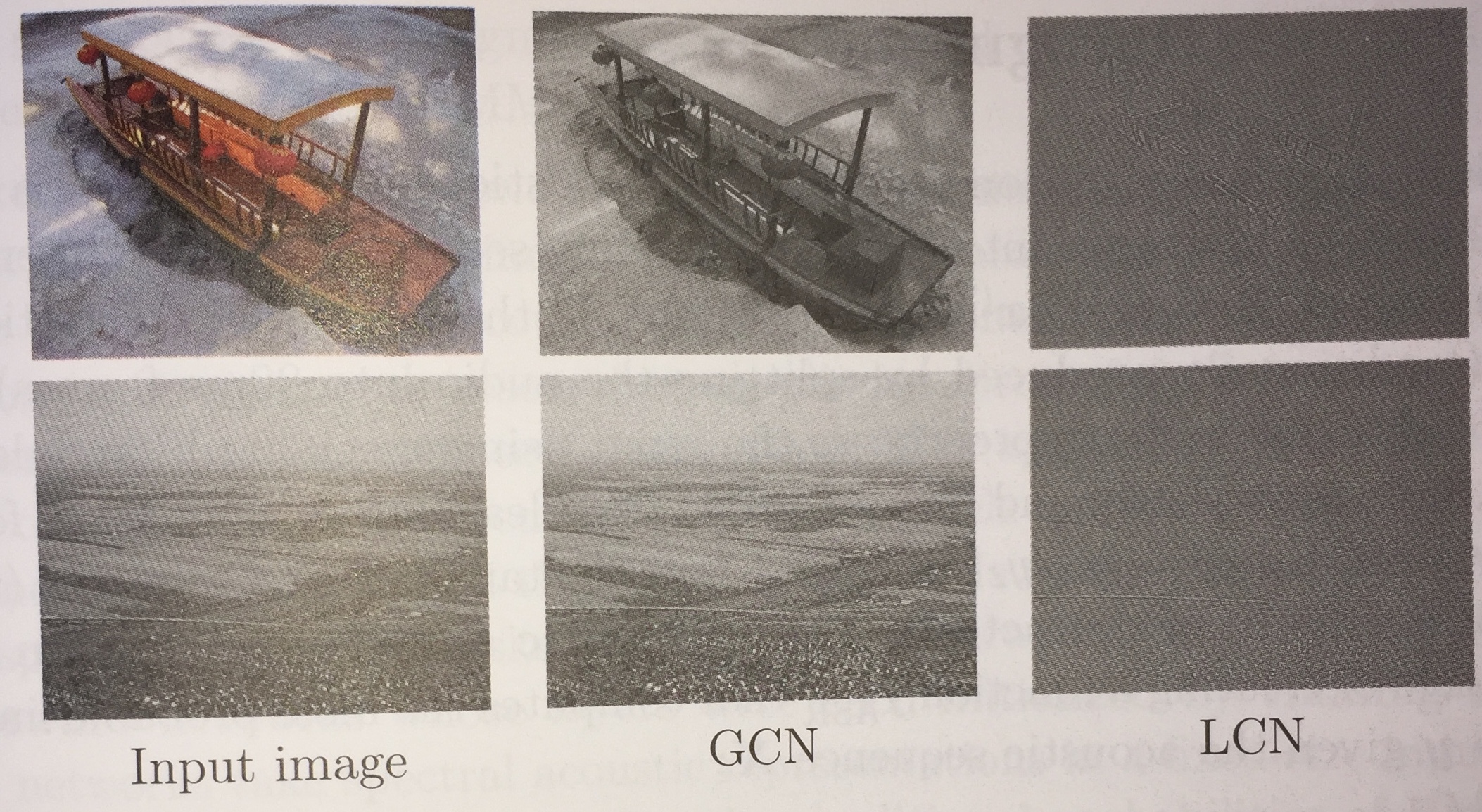
- Although, Global Contrast Normalization will ensure that there is a large difference between the brightness of dark and light areas within an image, it will often fail to highlight images features such as dark/light edges and dark/light corners in a light/dark region, something which might be useful for image classification, detection, etc.
- Local Contrast Normalization (LCN) can solve this problem by subtracting from each pixel a mean of nearby pixels and dividing by the standard deviation.
- Nearby could mean either an average over some rectangle centered at a given pixel, or could be a weighted Gaussian centered at the pixel. It can also be done independently/color channel.
- The above images from the book show the effects of GCN and LCN.
Dataset Augmentation
- One way to improve the generalization of a classifier is by increasing the size of the training set.
- This can be done by adding copies of the training examples that have been modified by transformations that do not change the class.
- Some example such transformations applicable in the computer vision setting are: random rotation, random translations, and random reflections.
- One can also randomly perturb the colors with noise or apply small geometric distortions.
Speech Recognition
- Speech recognition involves trying to map the acoustic signal of someone speaking into a sequence of text words of whatever was being said.
- The automatic speech recognition (ASR) task is to compute a map `f_{ASR}^\star` from `X = (vec{x}^{(1)},...,vec{x}^{(T)})`, a sequence of acoustic input vectors (say 20ms audio samples), to `vec{y} = (y_1, .., y_2)` the most probable target output sequence of words or characters.
`f_{ASR}^\star = arg max_{vec{y}} P^{\star}(vec{y}|\mathbf{X} = X)`.
- Here `P^{star}` is the true conditional distribution relating the inputs `X` to the targets `vec{y}`.
- From the late 1980s till around 2012, the state-of-the-art speech recognition systems combined HMMs and Gaussian Mixture Models (GMMs).
- GMMs (Bahl et al 1987) modeled the association between acoustic features and phonemes, HMMs were used to model the sequence of phonemes.
- The idea was that roughly when someone speaks their brain first computes a sequence of phonemes and then computes per phoneme how to make a sound. GMMs allow phoneme sounds to blend and overlap. So by modeling this in reverse we can figure out what was said.
Speech Recognition - Deep Models
- At the start of the time that the GMM-HMM model rose to prominence, neural networks achieved comparable phoneme error rates of 26% on the TIMIT (Texas Intrument-MIT) dataset (Garofolo et al 1993) of American male and female speakers as the GMM-HMM, but were not as popular because they were more complicated.
- Starting in 2009, as larger data models became available various researcher tried to replace the GMM component of the speech model with neural nets.
- One approach was to use a two layer network called a restricted Boltzman machine.
- Here we imagine having a fixed number of observable/visible sound outputs values `vec{v}` which are being produced by a set of hidden units `\vec{h}`
given an energy equation:
`E(vec{v},vec{h})=-vec{a}^{T}vec{v}-b^{T }vec{h}-vec{v}^{T}Wvec{h}`. From this one get a probability tof the form:
`P(vec{v},vec{h}) = 1/Z exp(-E(vec{v},vec{h}))` where `Z` is the partition function (an exponential sum of possible values of `vec{v},vec{h}` much like a softma)).
- Mohamed et al 2009, 2012 using this set up improved the phoneme error rate to 20.7 percent.
- Using NNs to model speaker specific features of the phonemes further improved the error rate (Mohamed et al 2011).
- The next major improvement for the phoneme recognition problem was to model the audio samples asa two dimensional image (one axis corresponding to time, the other to frequency of spectral components) and then to use CNNs to process the audio to figure out the phonemes (Saineth 2013).
- With these techniques NNs were performing better than the GMM-HMM framework which had not shown significant improvement for a decade despite larger data sets.
- Graves 2013 replaced the HMM component of the model with an LSTM RNN. Other deep models since have also replaced the HMM component getting the error rate down on TIMIT to less than 17.7%.
Natural Language Processing
- Natural Language Processing (NLP) is the use of human language such as English by a computer.
- Unlike a compiler situation where there might be a formally specified source and target computer language, natural languages
are often ambiguous (have multiple parsings of the same sequence), might not be context-free, etc., which make them harder to deal with.
- An example NLP task is machine translation: Read a sentence in one human language and translate it to another.
- Many NLP tasks are based on language models that define a probability distribution over sequences of words in a natural language.
- To build good networks in the NLP setting we need to process sequences of words, where each word is coming in general from a large vocabulary of words in some natural language.
- This means it is important to develop techniques to make models of these large, sparse discrete spaces as memory efficient as possible.
Language Models, `n`-grams
- A language model is a probability distribution over sequences of tokens in a natural language.
- One of the simplest such models is based on sequences of tokens of length `n` (an `n`-gram).
- When `n=1`, we say unigram; when `n=2`, bigram; and when `n=3`, trigram.
- By examining a large corpus of text, we can approximate the probability of a sequence `x_1, ..., x_n` as the number of times this sequence occurred in the corpus divided by the number of `n`-grams in the corpus.
- Using `n`-grams we can model the probability of an arbitrary sequence of tokens `x_1, ..., x_{\tau}` as:
`P(x_1, ..., x_{\tau}) = P(x_1, ..., x_{n-1})\prod_{t=n}^{tau}P(x_t| x_{t-n+1}, ..., x_{t-1})`.
- Usually, when one wants to make a `n`-gram language mode,l one goes over the data set computing both `n`-gram and `n-1`-gram frequencies (hence, allowing us to get their probabilities).
- From this we can compute `P(x_t| x_{t-n+1}, ..., x_{t-1})` as `(P(x_{t-n+1}, ..., x_{t}))/(P(x_{t-n+1}, ..., x_{t-1}))`.
- `n`-gram models have been popular since at least the early 1980s (Jelinek Mercer 1980).
Smoothing, Back-off, and Class-base Methods
- The problem with the set up of the last slide is what to do when the training corpus doesn't contain the sequence `x_{t-n+1}, ..., x_{t-1}`, and so `P(x_{t-n+1}, ..., x_{t-1}) = 0`. This can happen even in the unigram case if a real word just doesn't happen to be in the corpus.
- We don't want to divide by `0` in the equation of the last slide, so instead we smooth our `n`-gram probabilities. I.e., we take the `n-1` gram probabilities as `gamma` times the probability of the individual tokens plus `(1-gamma)` times the `(n-1)`-gram probability and we modify the probabilities of tokens so that all tokens have a minimal non-zero probability.
- Another issue is that if a given `n`-gram doesn't occur very often in our corpus our estimate for its probability might be bad. To handle this, we might use a threshold, and if the frequency of an `n`-gram is below a threshold, we use a backed-off model based on `n-1` gram probabilities to estimate its `n`-gram probability.
- A given `n`-gram comes from a space of size `|V|^n` where `V` is the vocabulary which might be of size `~ 10^5` or `~ 10^6`.
- So most `n`-grams are unlikely to occur in even a large corpus.
- To help solve this problem sometimes tokens/words are grouped into classes of similar meaning creating a class-based language model.
Neural Language Models
- Neural Language Models (NLM) are a language models built using neural nets.
- These are usually designed to try to overcome the curse of dimensionality problem mentioned at the bottom of the last slide for modeling natural language sequences.
- The idea is we use a neural net to map words (viewed as a 1-hot vector in a space of dimension the size of the vocabulary) into
a much smaller feature space of dimension usually on the order of `10^2` or `10^3`.
- This mapping is called a word embedding and we want to train it so that words that share similar properties are mapped close to each other in this much smaller space. For example, cat and dog share many properties and this would be reflected in their embedding vectors distance from each other.
- One way to train a word embedding is to use a skip-gram, a `2n+1`-gram where its middle word is missing. (Rather than a skip-gram one can also use a continuous bag of words (CBOW)).
- We train a low depth model consisting of an input layer (a 1-hot word), a hidden layer of size the target dimension, and an output softmax layer to predict the missing word.
- The embedding is the values of the hidden layer on a given input.
High Dimensional Outputs, Short Lists, Hierarchal Softmax
- A given output coordinate of the skip-gram the above process might compute is given by:
`a_i = b_i + sum_j W_{ij} h_j` for `i in {1, ..., |V|}` where `h_j` is the hidden unit `j`'s output
`hat{y_i} = (e^{a_i})/(sum_{i'=1}^{|V|} e^{a_{i'}})`
- So if `vec{h}` contains `n_h` elements then the above operation is `O(|V|n_h)`, so this operation dominates the computation time of most NLMs.
- (Bengio et al 2001, 2003, Swenk et al 2002 2007) propose a way to reduce this high computation cost by splitting the vocabulary into a short list `L` of high frequency words (handled by the NN) and a tail `T = V - L` of less frequent words which is just handled by an n-gram model. The neural net is then trained not only on `L` but also to predict the likelihood a word in the skip-gram come from the tail. If it is most likely to come from the tail the `n`-gram language model is used to predict it.
- Goodmann 2001 proposed a different approach where instead of having a single softmax layer one has a hierarchy of softmax layers.
- Training on this allows the net to build categories of words and categories of words of words.
Neural Machine Translation
- Early NN models for machine translation such as Allen 1987, Chrisman 1991, Forcada and Neco 1997 took a encoder decoder approach.
- Most systems compute the probability `P(t_1, t_2, ..., t_k | s_1, s_2, ..., s_n)` where `t_i` are the translated tokens and `s_j` are tokens in the source to be translated.
- The drawback of this is that sequences are of a fixed length.
- To overcome this, starting with Cho et al 2014, Sutskever 2014, and Jean et al 2014, RNNs systems were used.
- Using a fixed size vector to encode information about a long sentence can be difficult.
- One approach is to read the whole sentence or paragraph, and then produce translated words one at a time, each focusing on a different part of the input sentence to gather the meaning required to product the next word.
- This idea is behind attention based translators. (Bahdanau et al 2015).
- Such a system has three components:
- A process that reads the raw data and converts them to one feature vector/word read.
- A list of feature vectors storing the output of the reader.
- A process that exploits the content of the memory to sequentially perform a task, at each step having the ability put attention the content of a few memory elements. (This generates the translation.)


