


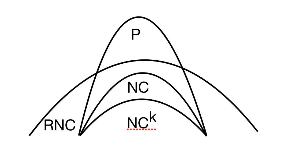
PRAM Sorting and Maximal Independent Set
CS255
Chris Pollett
Feb 27, 2019
CS255
Chris Pollett
Feb 27, 2019
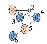
Greedy MIS:
Input: Graph G(V,E) with V = {1,..,n}
Output A maximal I contained in V.
1. I := emptyset
2. For v=1 to n do
3.     If Gamma(v) intersect I = emptyset then I := I union {v}.