Outline
- Scheduling
- Brent's Theorem
- Analyzing Multithreaded Computations
- Parallel For Loops
Introduction
- On Wednesday, we were talking about multithreaded computation.
- We started with an example program Fib(n) that computes the `n`th Fibonacci number, and we showed how to
parallelize it to a procedure P-Fib(n) using spawn and sync.
- We defined `T_P` to be the time needed for a multithreaded algorithm on `P` processors and `T_(infty)` to be the time it would
take if we had as many processors as needed to fully exploit the logical parallelism of the algorithm.
- We called `T_1` the work involved in the algorithm `T_(infty)` the span and `T_1/T_P` the speedup.
- We gave two inequalities: the work law: `T_P ge T_1/P`, and the span law: `T_P ge T_(infty)`.
- We said if `T_1/T_P = Theta(P)` we have linear speedup and if `T_1/T_P = P` we have perfect linear speedup.
- Using the span law, we showed if the slackness of the algorithm, `T_1/(P T_(infty))`, was less than one,
one can't get perfect linear speedup.
- Today, we are going to begin with techniques to schedule places with logical parallelism to processors.
Scheduling
- A multithreaded scheduler must schedule the computation with no advance knowledge of when strands will be spawned or when they will complete.
That is, the scheduler must operate online.
- A centralized scheduler (as opposed to a distributed one) knows the global state of the computation at any time.
- A greedy scheduler is a centralized scheduler that assign as many strands to processors as possible in each step.
- A complete step is a step in which at least P strands are ready to execute during a given step; otherwise, the step is incomplete.
- In a complete step a greedy scheduler assigns any `P` of the ready strands to processors.
Brent's Theorem (1974)
- The next result is a variant of a result of Brent 1974. In our context, it is due to Blumofe and Leiserson 1994.
- The work law says the best running time we could hope for is `T_P = T_1/P` and the span law says that the best running time we could
hope for is `T_P = T_(infty)`.
- The following theorem due to Brent modified for our parallel model shows that greedy scheduling is provable good in that it achieves the sum of these
two lower bounds as an upper bound.
Theorem. On an ideal parallel computer with `P` processors, a greedy scheduler executes a multithreaded computation with work `T_1` and span `T_(infty)` in
time
`T_P le T_1/P + T_(infty)`.
Proof of Brent's Theorem
We break the computation into complete and incomplete steps.
Consider the complete steps of the computation. In each complete step, the `P` processors perform `P` work. Suppose
that the number of complete steps was greater than `lfloor T_1/P rfloor`. Then the total work of the complete steps is at least
`P cdot(lfloor T_1/P rfloor + 1) = P lfloor T_1/P rfloor + P`
`= T_1 - (T_1 mod P) + P`
`> T_1`.
This is a contradiction because this would imply that the `P` processors perform more work than the computation requires. Hence, we have
that there are fewer than `lfloor T_1/P rfloor` complete steps.
Now consider an incomplete step. Let `G` be the DAG representing the entire computation. By replacing each strand of longer than unit time computations with a chain of unit time strands, we can assume each strand takes less than unit time. Let `G'` be the subgraph of `G` that has yet to be executed at the start of an incomplete step, let `G''` be the subgraph to be executed after the incomplete step. A longest path in a DAG must necessarily start at a vertex with in-degree 0. Since an incomplete step of a greedy scheduler executes all strands with indegree 0 in `G'` the length of the longest path in `G''` must be 1 less than the longest path in `G'`. So an incomplete step decreases the span of the unexecuted DAG by 1. Hence the number of incomplete steps is at most `T_(infty)`.
Since each step is either complete or incomplete, the theorem follows.
Quiz
Which of the following statements is true?
- The expected length of the longest streak in `n` coin flips is `Theta(\log n)`.
- We showed that if we chose `k = n/e` in our online hiring algorithm, then the algorithm always find the best candidate.
- The span law says: `T_P ge T_1/P`.
Optimality of Greedy Scheduling
Brent's Theorem allows us to show that greedy scheduling is close to optimal in the following sense.
Corollary. The running time `T_P` of any multithreaded computation scheduled by a greedy
scheduler on an ideal parallel computer with `P` processors is within a factor of 2 of optimal.
Proof. Let `T_P^star` be the running time produced by an optimal scheduler on `P` processors. The work and span
laws give: `T_P^(star) ge max(T_1/P, T_(infty))`. Brent's Theorem on the other hand implies:
`T_P le T_1/P + T_(infty)`
`le 2 cdot max(T_1/P, T_(infty))`
`le 2T_P^(star)`. QED.
Perfect Linear Speedup versus Slackness
Our next result shows that as a computation gets more slack it gets closer to having perfect linear speedup.
Corollary. Let `T_P` be the running time of a multithreaded computation produced by a greedy
scheduler on an ideal parallel computer with `P` processors. Then, if `P lt lt T_1 / T_(infty)` , we
have `T_P ~~ T_1/P`. That is, the speedup is approximately `P`.
Proof. Suppose `P lt lt T_1 / T_(infty)`, then `T_(infty) lt lt T_1/P`. By Brent's Theorem,
`T_P le T_1/P + T_(infty) ~~ T_1/P`. As the work law says `T_P ge T_1/P`, we conclude `T_P ~~ T_1/P`. This implies
the speedup is `T_1/T_P ~~ P`. QED.
Example. Suppose the slackness, `T_1/(P T_(infty))`, was greater than 10. Then the span, `T_(infty)` term in Brent's Theorem
is less than 10% of the the work/processor term. So if a computation runs on only 10 or a 100 processors, it doesn't make sense to value parallelism, `T_1/T_(infty)`, of 1000000 over parallelism of 10000 even with the factor of 100 difference.
Analyzing Multithreaded Algorithms
- Let's analyze the P-Fib(n) algorithm from Monday.
- We showed on Monday that `T_1(n) = Theta(phi^n)` where `phi = (1+sqrt(5))/2`.
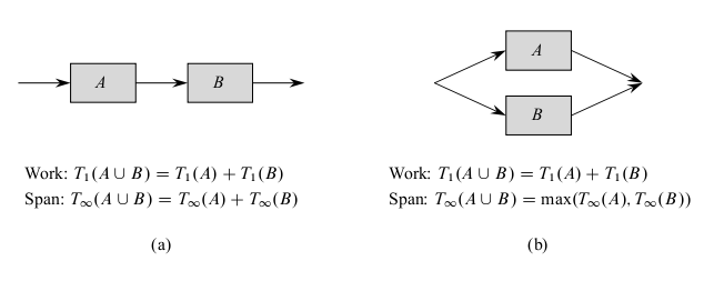
- The above diagram shows how to determine the span of a parallel computation DAG: Namely,
if two subcomputations are joined in series, their spans add to form the span of their composition; if
two subcomputations are joined in parallel, the span of their composition is the maximum of the spans of the two subcomputations.
- For P-Fib(n), the spawned call to P-Fib(n-1) runs in parallel with the call to P-Fib(n-2).
- So we can express the span of P-Fib(n) via the recurrence:
`T_(infty) (n) = max(T_(infty)(n-1), T_(infty)(n-2)) + Theta(1)`
`= T_(infty)(n-1) + Theta(1)`
which has solution `T_(infty) (n) = Theta(n)`.
- So the parallelism of P-Fib(n) is `(T_1(n))/(T_(infty)(n)) = Theta((phi^n)/n)`. This grows exponentially as `n` gets large.
- Hence, on parallel computers with a large fixed number `P` of processors, this algorithm will exhibit nearly perfect linear speedup for modest values of `n`.
Simulating Parallel For using Spawn and Sync
- A compiler can implement each parallel for loop as a divide-and-conquer subroutine using nested parallelism.
- For example, lines 5-7 can be implement with the call MAT-VEC-MAIN-LOOP(A, x, y, n, 1, n) where MAT-VEC-MAIN-LOOP is defined as:
MAT-VEC-MAIN-LOOP (A, x, y, n, i, i')
1 if i == i':
2     for j = 1 to n
3         y[i] = y[i] + a[i][j] * x[j]
4 else:
      mid = floor((i+ i')/2)
5     spawn MAT-VEC-MAIN-LOOP(A, x, y, n, i, mid)
6     MAT-VEC-MAIN-LOOP(A, x, y, n, mid + 1, i')
7     sync
Analyzing MAT-VEC(A, x)
- To calculate `T_1(n)` for MAT-VEC we just remove the parallel keywords and analyze the resulting code.
- Because of the doubly nested loops this gives, `T_1(n) = Theta(n^2)`.
- As we are converting parallel-for loops to spawn sync calls in a balanced fashion, the span to execute these calls will be the depth
of the tree of recursive calls and so logarithmic in the number of tree leaves, in this case `n`.
- More precisely, for a parallel loop with `n` iterations in which the `i`th iteration has span `iter_(infty)(i)`, the span is
`T_(infty)(n) = Theta(log n) + max_(1 le i le n) iter_(infty)(i)`.
- In the case of MAT-VEC, the first parallel for loop has span `Theta(log n)` as each iteration is `Theta(1)`. In the case of the second
parallel for loop, we have an inner serial for loop so get the span to be `Theta(n)`.
- Hence, the span of the whole algorithm will be `Theta(n)`, as it will be dominated by the second parallel for loop.
- The parallelism of this whole algorithm is thus `(Theta(n^2))/(Theta(n)) = Theta(n)`.


