Outline
- Properties of Degree 3 Bezier Curves
- De Casteljau's Method
- Recursive Subdivision
- Applications
- Piecewise Bezier Curves
- Notions of Smoothness
Properties of Degree 3 Bezier Curves
- Last day, we started talking about Bezier curves which are useful to specify shapes in two dimensions.
- Our goal is to eventually talk about surfaces, but for today we will continue exploring Bezier curves.
- Recall the equation for a Bezier curve is given by:
`\vec q(u) = B_0(u)\vec p_0 + B_1(u)\vec p_1 + B_2(u)\vec p_2 + B_3(u)\vec p_3`
where `B_i(u) = ((3),(i))u^i(1-u)^(3-i) `.
- We called the `B_i` blending functions. One property they have is the sum of the blending functions adds to `1`:
`\sum_{i=0}^3B_i(u) = \sum_{i=0}^3((3),(i))u^i(1-u)^(3-i) = (u+(1-u))^3 = 1`
- So `\vec q(u)` is always a weighted average of the four control points. From the definition of the `B_i` we also have `\vec q(0) = \vec p_0` and
`\vec q(1) = \vec p_3`
Blending Functions
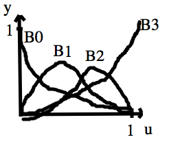
- The above graphs show us how much each of the blending functions is weighted as u varies from 0 to 1.
- By calculating the derivatives of the `B_i`'s and substituting in the values for 0 and 1 we find:
| `B'_0(0) = -3` | `B'_1(0) = 3` | `B'_2(0) = 0` | `B'_3(0) = 0` |
| `B'_0(1) = 0` | `B'_1(1) = 0` | `B'_2(1) = -3` | `B_3(1) = 3` |
- As `\vec q'(u) = B'_0(u)\vec p_0 + B'_1(u)\vec p_1 + B'_2(u)\vec p_2 + B'_3(u)\vec p_3`, this tells us that:
`\vec q'(0) = 3(\vec p_1 - \vec p_0)`
`\vec q'(1) = 3(\vec p_3 - \vec p_2)`
i.e., the fact mentioned on Tuesday that the curve starts off pointing in the direction of the line between `p_0` and `p_1` and end in the directions between `p_2` and `p_3`
De Casteljau's Method
- Using the derivative at the endpoints as was done on the last slide can help you draw a free-hand sketch of what a Bezier curve will look like.
- De Casteljau's method can be used to more easily find the values of `\vec q(u)`.
- Let `\vec p_0`, `\vec p_1`, `\vec p_2`, `\vec p_3` be the four points defining our degree 3 Bezier curve `\vec q(u)`.
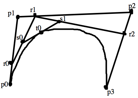
- We first form three new points `\vec r_0`,`\vec r_1`,`\vec r_2` from these `\vec p_i`'s using linear interpolation. i.e., via the euqations:
`\vec r_i = (1-u)\vec p_i + u\vec p_(i+1).`
- From these three points we form two more points `\vec s_0` and `\vec s_1` again by interpolation:
`\vec s_i = (1-u)\vec r_i + u\vec r_(i+1).`
- Finally, we set `\vec t_0 = (1-u)\vec \vec s_0 + u\vec \vec s_1`.
- Magically, (or just expand out the equations in terms or the original `\vec p_i`'s to see), it turns out
`\vec t_0` will be on the Bezier curve.
- Doing this for `u=1/2`, gives `\vec q(1/2) = 1/8 \vec p_0 + 3/8 \vec p_1 + 3/8 \vec p_2 +1/8 \vec p_3`.
Image of De Casteljau's Method
Recursive Subdivision
- It is much easier to draw lines than curves.
- So it useful to be able to come up with techniques to approximate Bezier curves with line segments.
- In order to do this, we will develop techniques to split a existing Bezier curve into two Bezier curves.
- If `\vec q(u)` is given by `\vec p_0`, `\vec p_1`, `\vec p_2`, `\vec p_3`, then one way to define two curves that together give all of `\vec q(u)` is to set:
`\vec q_1(u) = \vec q(u/2)` and `\vec q_2(u) = \vec q((u + 1)/2).`
- `\vec q_1(u)` and `\vec q_2(u)` are cubic because we substitued a linear factor in `\vec q(u)` which was cubic, but are they Bezier?
- Yes! You can mechanically verify that `\vec q_1(u)` is the Bezier curve with control points: `\vec p_0`, `\vec r_0`, `\vec s_0`, `\vec t_0` and `\vec q_2(u)` is the Bezier curve with control points: `\vec t_0`, `\vec s_1`, `\vec r_2`, `\vec p_3`.
- What if you wanted to make the split into two curves at point `\vec q(u_0)`? Instead, of `\vec q_1(u)` and `\vec q_2(u)` as above, you set
`\vec q_1(u) = \vec q(u_0u)` and `\vec q_2(u) = \vec q(u_0 + (1 - u_0)u).`
if we define `t_0 = q(u_0)` and define the `r_i`'s and `s_i`'s using `u_0` then `\vec q_1(u)` and `\vec q_2(u)` will be given by `\vec p_0`, `\vec r_0`, `\vec s_0`, `\vec t_0` and `\vec t_0`, `\vec s_1`, `\vec r_2`, `\vec p_3`.
Applications of Recursive Subdivision
- Given a Bezier curve, one way to draw it is to recursive split the curve into two halve curves and draw each of the halves.
- We keep splitting until the difference between the split Bezier curve and a straight line is less than some error `\delta`.
- We then draw a straight line for the Bezier curve.
- The Bezier curve is contained within the region specified by its four control points.
- So we thus want the approximating line segment `\bar(p_0p_3)` to be close to the points `p_1` and `p_2`.
- A quick and usually correct way to check for this is to see if `||\vec q(1/2) - 1/2(p_0 + p_3)|| < \delta`
- As we already said a couple slides ago `\vec q(1/2) = 1/8 \vec p_0 + 3/8 \vec p_1 + 3/8 \vec p_2 +1/8 \vec p_3`.
- Substituting this means checking that:
`||\vec p_0 - \vec p_1 - \vec p_2 - \vec p_3||^2 < (\frac{8\delta}{3})^2`.
Another Application of Recursive Subdivision
- Another use of recursive subdivision is intersection testing. i.e., You might want to see check if some Bezier surface is outside the viewing frustum and so does not need to be rendered.
- You can check if a ray intersects with a Bezier curve by checking first if the ray intersects with
the curves convex hull. If no, return false.
- If yes, split the Bezier curve into two halves and check for intersection on both halves.
- The recursion continues until we get to the line segment approximation level.
- Finally, if the ray and line segment intersect we actually output yes for the whole intersection test.
Piecewise Bezier Curves
- A single Bezier curve does not create an especially exciting shape; however, it is fairly straightforward to chain together several such curves to create whatever shape one wants in the plane.
- Curves made of a sequences of Bezier curves each tacked on to the last point of the previous one are called piecewise Bezier curves.
- Suppose we want to build `\vec q(u)` from `\vec q_1(u)` and `\vec q_2(u)`. Let
`\vec p_(i,0)`, `\vec p_(i,1)`, `\vec p_(i,2)`, `\vec p_(i,3)` where `i=1,2` be the control points for `\vec q_1`, `\vec q_2`.
- To join the two curves together we want `\vec p_(1,3) = \vec p_(2,0)`, so that `\vec q_1(1) = \vec q_2(0)`.
- If `\vec q(u)` is going to have a continuous first derivative at `u=1/2` we also need
`\vec q'_1(1) = \vec q'_2(0)` so that `\vec p_(1,3) - \vec p_(1,2) = \vec p_(2,1) - \vec p_(2,0)`.
- Two Bezier curves, tacked together will in general not have a continuous first derivative but if they do, then the resulting curve `\vec q(u)` will be said to be `C^1`-continuous.
Notions of Smoothness
- In some situation, having a continuous first derivative is useful.
- For example, if the Bezier curve is being used to describe the motion of an object. i.e.,
`u` is being used to measure time, then we might want the motion to appear smooth without sudden jerks or lurches.
- We define a curve to be `C^0` continuous if it is continuous on its domain, and for `k > 1` say a curve is `C^k` continuous if it is `C^(k - 1)` continuous and has continuous k derivative on its domain. A function is `C^\infty` continuous or smooth if it is `C^k` continuous for all `k`.
- A weaker notion than `C^1` continuity often suffices for drawing shapes, namely, geometric (`G^1`) continuity.
- `q(u)` defined piecewise from `\vec q_1(u)` and `\vec q_2(u)` is geometric continuous if `\vec p_(1,3) - \vec p_(1,2) = \alpha(\vec p_(2,1) - \vec p_(2,0))` for some constant alpha and neither difference is the zero vector.


