Outline
- Noteslidy
- Spline Curves
- Bezier Curves
- Degree 3 Bezier Curves
Using Slidy
- The slides for this class are HTML files which both validate as XHTML 1.1 and pass the WAVE Accessibility Checker.
- They are made to look like slides using a Javascript called Slidy.
- The following keystrokes do useful things in Slidy:
- h - help (see all the commands)
- f - fullscreen (gets rid of the links at the bottom of the window
- space - advance a slide
- left/right arrows - forward or back a slide
- up/down arrows - scroll within a slide
- a - show all slides at once for printing
- n - add a note to a slide in a given namespace (a student of mine Sriram Krishnan added this extension)
Seeing the Math in the Notes
- This semester I am using ASCIIMathML.js to display math equations in my slides.
- To see the equations you need to use a MathML capable browser such as Firefox 1.5 or greater or use Internet Explorer with MathPlayer
Spline Curves
- Throughout this course we are going to learn how to specify geometric shapes or figures within a computer.
- In order to do this, we will usual specify a collection of points (which can be represented in the computer
as int's or floats) together with an algorithm to
compute the shape from the points.
- To begin we will start in 2D world and consider curves.
- We would like to be able to specify curves using both a small number of points (so not requiring much storage)
and an easy to compute algorithm.
- Splines are smooth curves satisfying these properties.
- Smooth general means that the curve does not have any sharp bends or points.
- Splines allow for isolated points which are not smooth.
- The main classes of splines we will look at are Bezier Curves and B-spline curves.
Bezier Curves
- Bezier Curves were first developed by automobile designers to describe the shape of exterior car panels.
- They are named after Bezier who worked at Renault in France.
- Slightly earlier, de Casteljau had developed mathematically equivalent methods to define spline curves while
at Citröen.
- Today, we are going to look a little at degree 3 Bezier curves.
- Over the next couple of days, we will talk about curves of higher degree, extensions of these kinds of curves to surfaces
and how to implement these in OpenGL.
Degree 3 Bezier Curves
- A degree three Bezier curve will turn out to be a polynomial of degree 3.
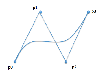
- It is specified by giving saying what its four control points `p_0`, `p_1`, `p_2`, `p_3` are.
- This curve has the property that it starts at `p_0` and ends at `p_3`.
- You can think of the points `p_1` and `p_2` as giving "something like" a gravitational pull on the straight line between `p_0` and `p_3`. The curve starts out at `p_0` with its tangent pointing towards `p_1`; it ends at `p_3` with it tangent aligned with `p_2`.
- We say that a curve interpolates a control point if the control point lies on the curves.
- In general, Bezier curves do not interpolate control points.
Definition of Degree 3 Bezier Curve
- A degree 3 Bezier curve is defined parametrically by a function `\vec q(u)`. i.e., as `u` varies between `0` to `1`, the values of `\vec q(u)`
sweep out the curve. The formula for the curve is given by:
`\vec q(u) = B_0(u)\vec p_0 + B_1(u)\vec p_1 + B_2(u)\vec p_2 + B_3(u)\vec p_3`
where `B_i(u) = ((3),(i))u^i(1-u)^(3-i) `.
- Note when we extend to higher degree we will define `B_i` for `i>3`. `\vec q` could be a vector in 2, 3, or more dimensions.
- The `B_i`'s are called blending functions and we will discuss more of their properties next day.


