Introduction

On Thursday, we talked about the Distributed Data Facility.
We talked about the different DRDA levels, user, remote unit of work, distributed unit of work, and distributed request.
We talked about IBM's implementation of the DRDA access requester: DB2 Connect.
We talked about how DDF can handle different character encodings
We talked about where DDF info is stored in DB2's catalogs.
Finally, we talked about the commands for accessing remote sites using DDF.
Today, we are going to look at connection pooling and the DDF and then start a new topic: SQL.

Connection Pooling

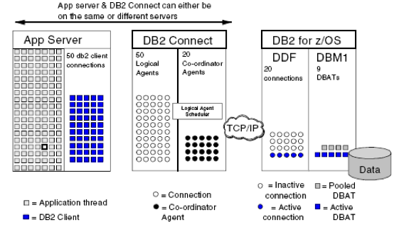
An image illustrating how connections are pooled on the app server, within DB2 connect, and on DB2 for z/OS

In order for the DDF to work efficiently, it needs a mechanisms for managing potentially thousands of concurrent connections.
This is done via a thread-pooling mechanism.
DB2 thread pooling operates by separating the distributed connections (in DDF) from the Data Base Access Threads (DBATs) that do the work (in DBM1).
A pool of DBATs is created for use by inbound DRDA connections.
A connection will make temporary use of a DBAT to execute a UOW, and then releases it back to the pool at commit time for another connection to use.
The result is a given number of inbound connections that require far fewer DBATs to execute the work within DB2.
On the application server and within DB2 connect pooling is also often used.
Each progressive form of connection pooling has the ability to reduce the connection demands on the next link in the chain.

Quiz

Which of the following statements is false?

In DDF several DB2 threads might be in the same enclave.
The WLM can assign dispatching priorities to stored procedure transactions based on the service class goals.
In the Distributed Unit of Work DRDA level, a two-phase commit protocol is needed.

Structured Query Language (SQL)

SQL is the de facto standard query language for relational database management systems (RDBMSs)
It allows you to specify WHAT data to retrieve, but not HOW
It is not merely a query language: you can query, but you can also define data structures, and control access to structures.

Relational Closure

Every SQL manipulation statement operates on a table and results in another table.
All operations native to SQL, therefore, are performed at a set level.
One retrieval statement can return multiple rows and one modification statement can modify multiple rows.
This feature of relational databases is called relational closure.
Relational closure is the major reason that relational databases, such as DB2, are generally easier to maintain and query.

DB2 Supported Data Types (High Level)

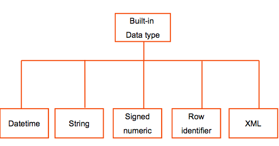
image showing the supported datatypes of DB2

DB2 also supports user-defined types.
Let's look at each of the above built-in data types of SQL in DB2 in turn...

Datetime Family

DATE: a three-part value that represents a year, month, and day in the range of 0001-01-01 to 9999-12-31.
TIME: a three-part value that represents a time of day in hours, minutes, and seconds, in the range of 00.00.00 to 24.00.00.
TIMESTAMP: a seven-part value that represents a date and time by year, month, day, hour, minute, second, and microsecond, in the range of 0001-01-01- 00.00.00.000000 to 9999-12-31-24.00.00.000000.

DB2 can convert between different regions formatting of dates and times. There are four supported output formats: ISO YYYY-MM-DD HH.MM.SS (24hr), USA MM/DD/YYYY Hour.Minutes am/pm, EUR DD.MM.YYYY HH.MM.SS (24hr), and JIS YYYY-MM-DD HH:MM:SS. For example,
SELECT EMPNO, CHAR(HIREDATE, USA) FROM EMP;

SQL also supports functions to get components out of dates. For example, DAYS(MY_DATE_VAR).

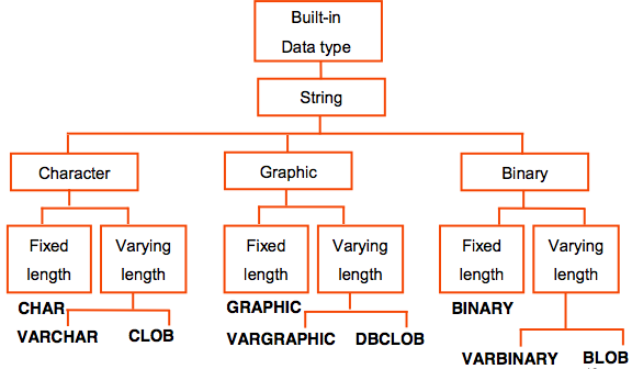
String Family of Datatypes

image showing the supported string datatypes of DB2

More Info about String Datatypes

Character strings contain text and can be either a fixed-length or a varying-length.
Graphic strings (think of as a pre-cursor to Unicode) contain double byte data, which can also be either a fixed-length or a varying-length.
Binary strings contain strings of binary bytes and can be either a fixed- length or a varying-length.
Variable length format incur a space overhead over the same value stored in its smallest fixed length format. For example, a three-byte string stored as a VARCHAR(3) will be two bytes longer than the same thing stored as a CHAR(3). For large tables this difference can be significant.
The VARCHAR, VARGRAPHIC, and VARBINARY data types have a storage limit of 32 KB. SO you need to use the appropriate Large Object type if you need to hold more data.

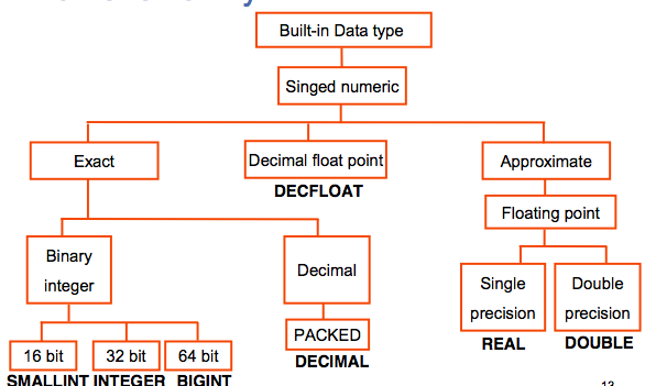
Numeric SQL Datatypes

image showing the supported numeric datatypes of DB2

More Numeric Datatypes

SMALLINT -- A small integer is a binary integer with a precision of 15 bits. The range is -32768 to +32767.
INTEGER or INT -- A large integer is a binary integer with a precision of 31 bits. The range is -2147483648 to +2147483647.
BIGINT -- A big integer is a binary integer with a precision of 63 bits. The range of big integers is - 9223372036854775808 to +9223372036854775807.
DECIMAL or NUMERIC DECIMAL(p,s) or NUMERIC(p,s) -- p is precision and s is scale: for packed decimal numbers with precision p and scale s. Precision is the total number of digits, and scale is the number of digits to the right of the decimal point.
DECFLOAT -- A decimal floating-point value is an IEEE 754r number with a decimal point. The position of the decimal point is stored in each decimal floating-point value. The maximum precision is 34 digits.
REAL -- A single-precision floating-point number is a short floating-point number of 32 bits.
DOUBLE -- A double-precision floating-point number is a long floating-point number of 64 bits.

Types of SQL Statement

As we've mentioned before SQL statements can be classified into three types:

DDL (Data Definition Language) -- used to define the data structures of a database. Consists of commands such as: CREATE, ALTER, and DROP.
DML (Data Manipulation Language) -- used to manipulate data stored in database data structures. Consists of commands such as: INSERT, UPDATE, and DELETE
DCL (Data Control Language) -- used to control who has privileges to access what data. Consists of commands such as: GRANT and REVOKE.

CREATE TABLE

Defines the structure of a table and its relationship to other tables in the database.

CREATE TABLE table_name ( column_defn1, column_defn2, ... )

column_defn: column_name column_type [DEFAULT expr]
  [column_constraint]

column_constraint: [CONSTRAINT constraint_name]
  {NOT NULL | CHECK (check-condition) | 
   PRIMARY KEY | FOREIGN KEY
   REFERENCES ref_table[(ref_column)] [ON DELETE action]}

action:
   NO ACTION | RESTRICT | CASCADE | SET NULL

NOT NULL mean the column cannot contain NULL values.
"CHECK (col1 > 20)" is an example of a CHECK with check condition. It means the value of col1 must be greater than 20.
PRIMARY KEY defines a primary key composed of the identified columns.
FOREIGN KEY REFERENCES define a referential constraint with another table.

Referential Integrity Illustration

CREATE TABLE DEPT ( DEPTNO CHAR(3) NOT NULL PRIMARY KEY, DEPTNAME VARCHAR(32), ... );

CREATE TABLE EMP ( EMPNO CHAR (6),
   DEPTNO CHAR(3),... 
   CONSTRAINT FK FOREIGN KEY (DEPTNO) 
     REFERENCES DEPT ON DELETE SET NULL);

A foreign key constraint specifies a relationship (a referential integrity (RI) constraint) between two tables: the parent table and the child table.
As long as the foreign key constraint is in effect, the system guarantees that, for each in the child table with a non-null value in all of its foreign key columns, there is a row in the parent table with a matching value in the parent key.
The RI relationship is recorded in the SYSIBM.SYSFOREIGNKEYS catalog table.
ON DELETE SET NULL means that if a department is deleted from DEPT, then all of the rows with that department will have their value for the DEPTNO column set to NULL.
ON DELETE CASCADE would have meant these rows would be deleted as well, when the given DEPT row was deleted
ON DELETE RESTRICT would prevent the DEPT row from being deleted until all EMP rows that reference it have either been changed or removed.
ON DELETE NO ACTION would prevent the deletion of the parent row as well. RESTRICT does its check before cascaded updates and deletes take effect; whereas, NO ACTION check after they take effect.

Table Examples

CREATE TABLE BOOK (
   BOOKNO INTEGER NOT NULL PRIMARY KEY,
   TITLE VARCHAR(100),
   AUTHOR VARCHAR(100));

CREATE TABLE MEMBER (
   CARDNO INTEGER NOT NULL PRIMARY KEY,
   NAME VARCHAR(100), 
   CITY VARCHAR(100));

NULL

NULL is used in SQL to represent a missing (unknown) or inapplicable values.
Computations involving null values result in null values. For example, 1 + NULL = NULL.
Aggregate functions vary in how they handle null values. For example, AVG does not include null values when computing averages; COUNT(*) includes rows of null values in its tally.
"column IS NULL" is used to test whether a column content is null.
A null value introduces three-value logic for Boolean operators: The result of "FALSE OR NULL" is NULL; "TRUE AND NULL" is NULL; NOT NULL is NULL

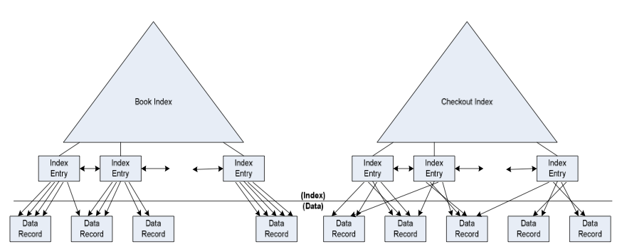
CREATE INDEX

CREATE [UNIQUE] INDEX ON 
table_name(column_list) [CLUSTER | NOT CLUSTER]

An index is usually created to speed up the processing of queries against the base table.
Each row in the index table contains a index key value and all its data table RIDs (physical Row ID).
An UNIQUE specification in the CREATE INDEX will guarantee that no two rows may share the same index value. INSERT or UPDATE operation which introduce duplicate values are rejected.
When CLUSTER is specified, the physical organization of the data mirrors the index as closely as possible. The retrieval of the data page via a clustered index results into fewer random I/O and thus has better performance.
An index is like a table which takes physical storage. The cost of maintaining an index will also slow down data modifications (INSERT, UPDATE, DELETE).

Index Examples

CREATE UNIQUE INDEX BOOKINDEX ON BOOK(BOOKNO)
  CLUSTER; 

CREATE INDEX CHECKOUTINDEX ON CHECKOUT(BOOKNO);

ALTER

The ALTER TABLE statement is used to add a column to an existing table, to increase the length of a VARCHAR column, or to add or drop some other table property such as a constraint.

ALTER TABLE Tablename {
 ADD {column_defn | table_constraint} |
 ALTER column_name SET DATA TYPE data_type |
 DROP {PRIMARY KEY | {FOREIGN KEY | CHECK |
 CONSTRAINT} constraint_name}}

ALTER INDEX Indexname{ {CLUSTER | NOT CLUSTER} |
 {ADD COLUMN (column_name)}}

DROP

The DROP command can be used to delete a table or an index. The syntax looks like:

DROP TABLE table_name
DROP INDEX index_name

Dropping a table also drops all indexes and views defined on the table.
A user might want to drop an index if a large number of data modifications (INSERT, UPDATE, DELETE) are planned. The user can drop the index (to avoid the index maintenance) and then re- create it after the high volume of data changes is complete.
Dropping an index might affect constraints that are enforced by the index. For example, if a primary index is used to enforce a unique constraint, then the constraint must be dropped before dropping the index.

Overview of SQL

Outline