We now consider a second model in which learning algorithms are known: neural nets.
It is generally believed that mental activity consists primarily of electrochemical activity in networks
of brain cells called neurons.
One of the first mathematical models of a neuron was devised by McCulloch and Pitt (1943). This paper is also the paper most frequently cited as defining finite automata.
Since the publication of this model of neuron, much medical work has been done on the specifics of how neurons work.
AI workers on the other hand have been more interested in the abstract properties of neural networks, such as their ability to perform distributed computation, to tolerate noisy inputs, and to learn.
We will now consider some of these properties.
Neural Network Structure
Neural networks are composed of nodes or units called neurons which are connected by directed links.
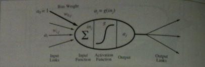
A basic neuron looks like the above image.
A link from unit `i` to unit `j` serves to propagate the activation `a_i` from `i` to `j`. (Think of this as something like an electrical signal).
Each link has a numeric weight `w_(ij)` associated with it, which determines the strength and sign of the connection.
We will assume each unit has a dummy input `a_0 = 1` with an associated weight `w_(0,j)`.
To compute the output of unit j
`j` first computes a weighted sum of its inputs:
`i\n_j = sum_(i=0)^n w_(i,j)a_i`.
Then, it applies an activation function `g` to this sum to derive the output:
`a_j = g(i\n_j) = g(sum_(i=0)^n w_(ij) a_i)`
This output could then be fed into several other neurons.
Perceptrons
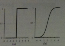
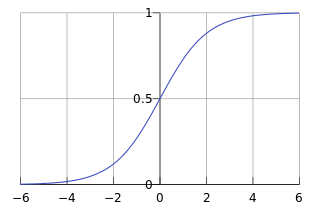
The activation function `g` is typically either a hard threshold or a logistic function (see above image).
In the former case the neuron would be called a perceptron, in the later case, a
sigmoid perceptron.
Making Networks
There are two common ways to connect neurons together to make networks: make connections in only one
direction without back lines (a feed-forward network) or to allow output to go back and serve as inputs (a recurrent network).
Networks that use the latter approach can exhibit oscillatory or even chaotic behavior, so are harder to analyse (probably more realistic).
So we will focus on feed-foward networks for now.
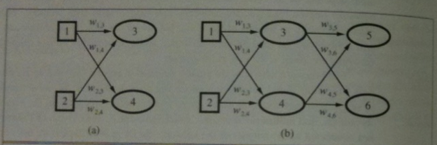
Feed-forwards networks are usually arranged into layers such that each unit receives input from only units in the immediately preceding layer.
Layers which are not directly connected with inputs or outputs are called hidden layers.
The above image shows a single layer of perceptrons on the left and a multi-layer network with so-called hidden layers
which are not connected to inputs or outputs directly.
We will start by considering learning algorithms for single-layer networks then move on to the multi-layer, feed-forward network case.
div class="slide">
What can a Perceptron Compute?
A network with all the inputs connected to units whose outputs are the final outputs is called a single-layer neural network,
or a perceptron network.
The left image on the previous slide is an example.
If we want to compute a function whose output is an `n` bit number with such a network, we would need to use one perceptron unit
for each output.
So to understand the power of perceptron networks, it suffices to understand what boolean-valued function a single perceptron is able to compute.
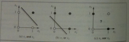
Suppose we had two inputs `x_1` and `x_2` with activations `a_1` and `a_2`. Then the first operation we use to compute the output of the perceptron is to compute a weighted sum of the inputs `w_(00) + w_(10)a_1 + w_(20)a_2`. Recall `w_(00)a_0` where `a_0` was always 1 was a dummy input line.
Applying a threshold at some number `t`, says when `w_(00) + w_(10)a_1 + w_(20)a_2 ge t` have the output be one value (say 1) and otherwise have it be another value (say 0).
Notice `w_(00) + w_(10)a_1 + w_(20)a_2 = t` for fixed `t` and `w_(i0)`'s is the equation of a line in the `a_i`'s.
Such a line could be used to separate the 0 and 1 output values of an AND or OR function as we see in the above image, but it could not be used to separate
the 0 and 1 output values of the parity (XOR) function.
In general, perceptron networks can only learn linearly separable functions.
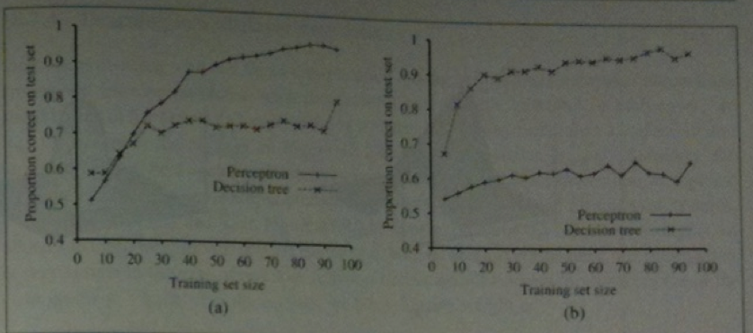
Perceptron Networks compared to Decisions Trees
Consider the majority function. It returns 1 if the majority of its inputs are 1 and 0 otherwise.
The left image above shows the training set size versus the proportion of correct answers on a test set for
both decision trees and perceptrons learning this function.
As we can by this example, with a smaller training set, the perceptron network was able to learn this function better
than using decision trees.
So there are still some reasons why we might be interested in studying perceptron learning.
The right image above, shows a problem where decision trees do better (the will wait for a seat a restaurant problem). This is
closer to a parity function.
In any case, we are interested in how to learn the weights we should use in a perceptron network.
This will also serve to help understand the general feed-forward case.
Quiz
Which of the following is true?
`P(cause|effect) = P(effect|cause)`.
Mean-based, hierarchal clustering is a supervised learning algorithm.
One way to implement Importance(A, examples) in the decision tree learning algorithm is to use Gain(A).
Sigmoid Perceptron
Recall before we said that the activation function `g` is often taken to be a threshold function or a logistic function.
The logistic function or sigmoid curve is defined as: `Logistic(t) = frac(1)(1+ e^(-t))`.
We can see it plotted above.
Notice it is very similar to a threshold function, but has the virtue of being differentiable.
We can view the sum that we compute when trying to find the value of a perceptron as being the dot product: `vec(w) cdot vec(x)`. For
now, we'll abuse notation and conflate `vec(x)` with the activations `vec(a)`.
A sigmoid perceptron (as a function) with weight vector `vec(w)` then can be defined as
`h_(vec(w))(vec(x)) = Logistic(vec(w) \cdot vec(x)) = frac(1)(1+ e^(-vec(w) \cdot vec(x)))`
Learning the Weights of a Sigmoid Perceptron
Recall a training set `E` consists of examples of the form `(vec(x), y)` where `vec(x)` are the inputs and `y` is
the output (0 or 1).
The process of fitting the weights of our logistic perceptron to this example set is called logistic regression.
The error or loss that a `h_(vec(w))` makes on the training set `E` can be calculated as:
`Loss(vec(w)) = sum_((vec(x), y) in E)(y - h_(vec(w))(vec(x)))^2`
Squaring is our cheap way of ensuring we are always adding nonnegative numbers.
We want to make this function of `vec(w)` as close to 0 as possible.
Recall one way to find the minimum of a function `f(x) = y` is to start with an initial guess of `x_0`, compute the tangent line to `(f(x_0))` and its derivative. See the sign of the derivative and move in that direction. Then repeat.
We want to take the same approach with the loss function above.
Learning the Weights Continued
To compute where the tangent hyperplane hits the axis to do our steepest descent method we need to compute the gradient of the Loss function.
Let `g` be the logistic function and `g'` its derivative.
For a single example (term in the Loss sum), the `i`th component of the gradient is:
`frac(del)(del w_i)Loss(vec(w)) = frac(del)(del w_i)(y - h_(vec(w))(vec(x)))^2`
`\quad = 2(y - h_(vec(w))(vec(x))) times frac(del)(del w_i)(y - h_(vec(w))(vec(x)))`
`\quad = -2(y - h_(vec(w))(vec(x))) times g'(vec(w) cdot vec(x)) times frac(del)(del w_i) vec(w) cdot \vec(x)`
`\quad = -2(y - h_(vec(w))(vec(x))) times g'(vec(w) cdot vec(x)) times x_i`.
One can verify that the derivative of the logistic function satisfies `g'(t) = g(t)(1- g(t))`.
Substituting this into the last line above gives us an update rule for weight `w_i`:
`n\ewW_i := w_i + alpha (y - h_(vec(w))(vec(x))) times h_(vec(w))(vec(x))(1 - h_(vec(w))(vec(x))) times x_i.`
So to compute the weights of our perceptron, we start with an initial guess of each of the `w_i`'s. Then for each `i` and each training set item
`(vec(x), y)` we calculate a `n\ewW_i` based on the weights so far. These `n\ewW_i`'s become the `w_i`'s for the next training example considered.
We go through the whole training set in the way. If the values of the weight seem
to be still fluctuating we run through the training set again until we get the desired/achievable stability.
Notice `\alpha` in the above. This could be set to a constant such as the one we get when taking derivatives. If so, we are using
a fixed rate learning ratio. Such a ratio, might prevent or slow convergence of our algorithm. The book gives an example where using a temperature-like schedule
of `alpha(t) = 1000/(1000+t)` where `t` is the number of iterations performs better.
Feed-Forward Networks
Before we discuss how to do learning in feed-forward networks, let's look at how
feed-forward networks can compute more complicated functions than perceptron networks.
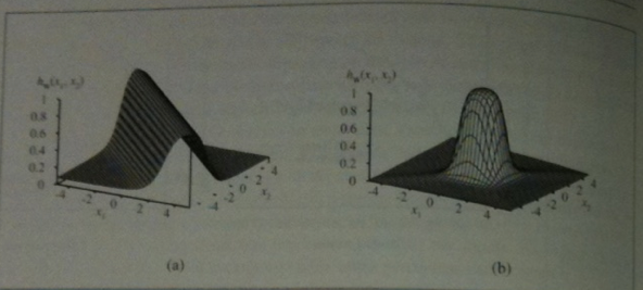
Recall a sigmoid perceptron layer will generally split one's space by a hyperplane into
a "low" region with values close to 0 and a "high" region with values close to 1.
We could imagine combining two thresholds one a value `t` which causes a transition from low to high with another threshold `t' > t` which causes a transition from high to low (weights would be opposite sign of the first one). This would give a network with a ridge as seen in the image above on the left.
Combining two more perceptrons function with perpendicular hyperplanes gives a spike as seen on the right. So in at most four layers we can build a spike.
Combining spikes allows us to compute whatever surface/function we want.
Feed-Forward Learning
To learn with feed-forward networks we want to use the same sort of gradient descent method we
used in perceptron learning.
In order to see how this will work, lets look at the outputs of the multilayer neural net given on the first slide.
As an example,the output activation for unit 5 can be calculated as
`a_5 = g(w_(05) + w_(35)a_3 + w_(45)a_4)`
We can in turn expand `a_3` and `a_4` to get:
`a_5 = g(w_(05) + w_(35)g(w_(03) + w_(13)x_1 + w_(23)x_2) + w_(45)g(w_(04) + w_(14)x_1 + w_(24)x_2))`
In other words, any output value can by be rewritten as function of only the input values.
Unfortunately, this function can be highly nonlinear, so computing how the Loss affects an individual gate is harder.
In general our algorithm will now be a kind of nonlinear regression.