Outline
- Inference
- Independence
- Baye's Rule
Introduction
- On Monday, we began talking about reasoning in the presence of uncertainty.
- We described a Decision Theory agent which tries maximize its expected utility.
- We introduced the concept of sample spaces, elements and events in sample spaces.
- We then described how distributions on variables can be used to come up with probability for
propositional formulas based on these variables.
- Today, we begin by looking at inference in a probabilistic setting.
Probabilistic Inference
- Consider a domain consisting of the three Boolean variables: Toothache, Cavity, Catch (dentist probes catches in mouth):
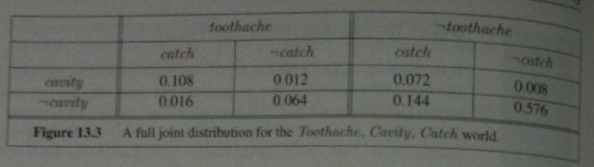
- Notice the probabilities in the full distribution sum to 1.
- There are six possible worlds in which `cavity vv t\o\othache` holds so it probability is: 0.108 + 0.012 + 0.008 + 0.016 + 0.072+ 0.064 = 0.28
- Often one wants to extract the distribution over some subset of variables or a single variable. For example, adding the entries in the first row gives the unconditional or marginal probability of cavity: 0.108+ 0.012 + 0.072 +0.008 = 0.2
- This process is called marginalization or summing out.
- The general rule for summing out any sets of variables `Y` and `Z` is:
`vec P(Y) = sum_(z in Z) vec P(Y,z).`
- For example, we just calculated `\vec{P}(Cavity) = sum_(z in \{Catch, T\o\othache\})\vec{P}(Cavity,z)`.
- I am writing `\vec{P}` when we are talking about the distribution rather than a probability.
- If we are dealing with conditional probabilities instead of joint probabilities, we get the following rule called
conditioning: `vec{P}(Y) = sum_z vec{P}(Y|z)P(z)`.
- Both of these rules are useful for derivations involving probability expressions.
Example of Computing Probabilities using Conditioning
- Using our definition for conditional probabilities from last day we can compute:
`P(cavity|t\o\othache) = frac(P (cavity ^^ t\o\othache) )(P(t\o\othache)) = frac(0.108 + 0.012)(0.108 + 0.012 + 0.016 +0.064) = 0.6` and
`P(neg cavity|t\o\othache) = frac(P (neg cavity ^^ t\o\othache) )(P(t\o\othache)) = frac(0.016 + 0.064)(0.108 + 0.012 + 0.016 +0.064) = 0.4`
- As you expect, these sum to 1. Notice that `frac(1)(P(\t\o\othache))` appears in both of these. We can treat it as a normalization constant `\alpha` for the distribution `\vec P(Cavity |t\o\othache)` ensuring that it adds up to 1
- So we have:
`\vec(P)(Cavity |t\o\othache) = \alpha \vec(P)(Cavity, t\o\othache)`
`quad = \alpha [\vec(P)(Cavity, t\o\othache, catch) + \vec(P)(Cavity, t\o\o\thache, neg catch)]`
`quad = \alpha[langle 0.108, 0.016 rangle + langle 0.012, 0.064 rangle] = \alpha langle 0.12, 0.08 rangle = langle 0.6, 0.4 rangle`
- So we can calculate `\vec(P)(Cavity |t\o\othache)` even if we don't know the value of `P(\t\o\othache)`, we just need to divide the last vector by the sum 0.12 + 0.08.
- Using this we can extract a general inference procedure: Begin with the case in which the query involves a single variable, `X` (Cavity in our example). Let `\vec(E)` be the list of evidence variables (Toothache in our example). Let `vec(e)` be the list of observed values for them, and let `Y` be the remaining unobserved variables (Catch in our case). The query is `\vec(P)(X | \vec(e))` and can be evaluated as:
`vec(P)(X|vec(e)) = \alpha vec(P)(X, vec(e)) = alpha sum_vec(y) vec(P)(X,vec(e),\vec(y))`
- Given the full joint distribution, this equation can answer probabilitic queries for discrete variables. It doesn't scale though: It require a table of `O(2^n)` size and so it take `O(2^n)` time to compute.
Independence
- Suppose we added to our three variables a fourth variable Weather to get the full joint distribution
`vec(P)(T\o\othache, Catch, Cavity, Weather)`. This table now has `2 times 2 times 2 times 4 = 32 entries`, four "editions"
of the table of the earlier slide one for each kind of weather.
- What relationship do these editions have to each other and to the original three-variable table?
- For example, how are `P(t\o\othache, catch, cavity, cloudy)` and `P(t\o\othache, catch, cavity)` related?
- Using the product rule we know:
`P(t\o\othache, catch, cavity, cloudy) = P(cloudy | t\o\othache, catch, cavity) P(t\o\othache, catch, cavity)`
- It is likely that the weather does not influence the dental variables. So it is safe to say:
`P(cloudy | t\o\othache, catch, cavity) = P(cloudy)`.
- A similar equation exists for every entry in
`\vec(P)(T\o\othache, Catch, Cavity, Weather)` so we get:
`\vec(P)(T\o\othache, Catch, Cavity, Weather) = \vec(P)(T\o\othache, Catch, Cavity)\vec(P)(Weather)`
- This property is called independence. In our case, the weather is independent of our dental problems
- Independence means a full joint distribution can often be factored into separate disjoint distributions. Independence can
often help reduce the size of the domain representation and complexity of the inference problem.
Baye's Rule and Its Use
- We already defined the product rules: `P(a ^^ b) = P(a | b)P(b)` and `P(a ^^ b) = P(b | a)P(a)`.
- Equating the two right hand sides gives us:
`P(b|a) = frac(P(a|b)P(b))(P(a))`
- This is called Baye's rule.
- Baye's rule is used quite often in AI systems. The reason is that although `P(b|a)` might be hard to directly calculate the three terms on the right are often easier to determine
- For example, we want to know the most likely cause of some effect. We could consider each cause and estimate:
`P(cause | effect) = frac(P(effect|cause)P(cause))(P(effect)).`
- `P(effect | cause)` quantifies the relationship in the causal direction, whereas `P(cause | effect)` describes the diagnostic direction.
- For example, a doctor often knows `P(symp\t\oms | disease)` but wants to calculate the disease that is causing the symptoms.
- So if the doctor knows that 70% of people with meningitis have stiff necks and the odds of meningitis are 1/50000 and the odds
of a stiff neck are 1/100. Then the odds of meningitis given a stiff neck are (.7 * 1/50000)/0.01 = 0.0014.
Probabilistic Agent Example
- Recall the Wumpus World game is played on a 4x4 grid starting at the lower left square.
- We want to find the gold, avoid pits and the Wumpus (neither of which move), and leave the world with the gold.
- Our knowledge about the world is given by sensors which can detect a breeze, a glitter, a stench, or a scream (if wumpus dies) in the adjacent square.
- In one turn, we can move forward, turn left/right, grab gold, and shoot.
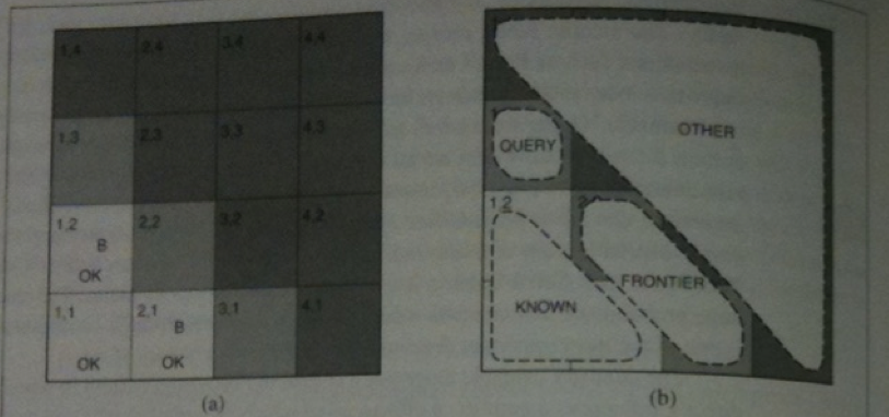
- The above possible world might represent a situation that could cause a purely logical agent to get stuck the three available squares that have not been
visited all might contain a pit. So which should we choose?
- We would like to use probabilities to choose the one least likely to contain a pit.
Modeling the Problem
- As in the logical case we will use the following variables:
- `P_(ij)` - represents square `(i,j)` has a pit.
- `B_(ij)` - represents `(i,j)` is breezy.
- To figure our what to do next we need to specify the full joint distribution
`vec P (P_(11), ..., P_(44), B_(11), B_(12), B_(21))`.
- This can be calculated using
`vec P (P_(11), ..., P_(44), B_(11), B_(12), B_(21)) = vec P(B_(11), B_(12), B_(21)|P_(11), ..., P_(44)) vec P(P_(11), ..., P_(44))`
- Each square contains a pit with probability 0.2 independently of all the other squares.
- So we have:
`vec P(P_(11), ..., P_(44)) = prod_(i,j =1,1)^(4,4) vec P (P_(ij))`.
- If the wumpus world has exactly `n` pits this gives:
`P(P_(11), ..., P_(44)) = (0.2)^n(0.8)^(16-n)`.
More Modeling the Problem
- We abbreviate by `b` the observed breeze information `neg b_(11) ^^ b_(12) ^^ b_(21)`.
- We abbreviate by `known` the squares we know pit info about `neg p_(11) ^^ neg p_(12) ^^ neg p_(21)`
- We are interested in queries such as `vec P(P_(13) | known, b)` : How likely is that (1,3) contains a
pit given the observations so far?
Answering the Question
- To answer the query we want to sum over entries from the full joint distribution.
- Let `Unknown` be the set of `P_(ij)` variables for squares other than `Known` squares and the query square.
- So as in our conditioning example earlier we have:
`vec P(P_(13) | known, b) = alpha sum_(unknown) vec P(P_(13), unknown, known, b)`
- There are 12 unknown squares, so the above sum contains 4096 terms.
- Not all squares are relevant to the probability on the left. For example `(4,4)` does not affect whether `(1,3)` has a pit.
- Let Frontier denote the pit variables that are adjacent to visited squares. i.e., (2,2) and (3,1).
- Let Other be the pit variables for the other unknown squares (10 in this case).
- We can manipulate the sum above to make use of the fact that the observed breezes are conditionally independent of the other variables, given the known, frontier,
and query variables:
`vec P(P_(13) | known, b)`
`= alpha sum_(unknown) vec P(P_(13), known, b, unknown)`
`= alpha sum_(unknown) vec P(b|P_(13), known, unknown) vec P(P_(13), known, unknown)`
`= alpha sum_(\f\rontier)sum_(other) vec P(b|known,P_(13), \f\rontier, other) vec P(P_(13), known, \f\rontier, other)`
`= alpha sum_(\f\rontier)sum_(other) vec P(b|known,P_(13), \f\rontier) vec P(P_(13), known, \f\rontier, other)`
- The last step uses the conditional independence.
- The first term above does not depend on the Other variables, so we can move the summation inwards giving:
`vec P(P_(13) | known, b)`
`= alpha sum_(\f\rontier)vec P(b|known,P_(13), \f\rontier)sum_(other)vec P(P_(13), known, \f\rontier, other)`
- By the independence of pit variables, we can factor the right hand sum and reorder things:
`vec P(P_(13) | known, b)`
`= alpha sum_(\f\rontier)vec P(b|known,P_(13), \f\rontier)sum_(other)vec P(P_(13))P(known)P(\f\rontier)P(other)`
`= alpha P(known) P(P_(13)) sum_(\f\rontier)vec P(b|known,P_(13), \f\rontier)P(\f\rontier)sum_(other)P(other)`
`= alpha' P(P_(13)) sum_(\f\rontier)vec P(b|known,P_(13), \f\rontier)P(f\rontier)`
- In the last step we use `sum_(other) P(other) = 1`.
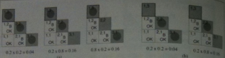
- The above sum has just four terms.
- `vec P(b|known,P_(13), \f\rontier)P(f\rontier)` is 1 when the frontier is consistent with the breeze observation and 0 otherwise.
- So we sum over the logical models that are consistent with the known facts.
- This gives us the models shown in the figure above.
- Working it out, we have:
`vec P(P_(13) | known, b) = alpha' langle 0.2 (0.04 +.16 +.16), 0.8 (0.04 +0.16) rangle approx langle 0.31, 0.69 rangle`


