Outline

• Finish Cord Cutting
• The LCS Problem

Introduction

• On Monday we started talking about Dynamic Programming as a technique to solve optimization problems.
• We said developing dynamic programming algorithms is often done by following four step: (1) Characterize the structure of an optimal solution, (2) recursively define the value of an optimal solution, (3) compute the value of an optimal solution, typically bottom up, and (4) use that to construct the optimal solution.
• We then introduced the rod cutting problem. This was to find the optimal way to cut a rod into integral pieces so that the price for these pieces could be maximized.
• We gave a recursive algorithm not using dynamic programming to solve this problem.
• Let's analyze this solution and then see how to make it go faster using dynamic programming...

Non-DP Cord-Cutting Analysis

Here is our cord-cutting code from Monday:

CUT-ROD(p,n)
1 if n == 0
2     return 0
3 q = - infty
4 for i = 1 to n
5     q = max( q, p[i] + CUT-ROD(p, n-i ))
6 return q

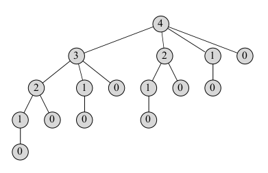
• It is inefficient in that CUT-ROD calls itself recursively over and over again with the same parameter values.
• The tree above shows the recursive calls made when `n = 4`. The node values represent the size of the sub-problem being called. Notice we calculate 2 and 1 several times.
• Let `T(n)` denote the total number of calls made to CUT-ROD when the second parameter is `n`.
• So `T(0) = 1` and `T(n) = 1 + sum_(j=0)^(n-1) T(j)`.
• By induction, one can show `T(n) = 2^n`, so this algorithm is very slow and takes a lot of space!

Rod-Cutting via Dynamic Programming

• Dynamic Programming uses additional memory to store values of the sub-problems so we don't have to recompute them.
• It is an example of a time-memory trade off -- we sacrifice memory for a quicker run-time.
• There are two equivalent ways to implement a dynamic programming approach: top-down with memoization and bottom-up.
• "Memoize" means we remember while we are doing the recursion what sub-problems we have computed previously
• In the bottom-up approach, we often rely on their being "natural sizes" for sub-problems. We sort the subproblems by size and solve them beginning with the smaller problems first. That way if a bigger problem relies on a sub-problem we have the solution to that sub-problem ready.

MEMOIZED-CUT-ROD

Here is the pseudo-code for the top-down approach. We use the array `r` to remember solutions to sub-problems. Before we compute a sub-problem we check if `r` has a value, if it does, we return what's stored in `r`; otherwise, we compute sub-problem.

MEMOIZED-CUT-ROD(p,n)
1 let r[0..n] be a new array
2 for i = 0 to n
3    r[i] = -infty // initialize subproblem solutions to sentinel value
4 return MEMOIZED-CUT-ROD-AUX(p,n,r)

MEMOIZED-CUT-ROD-AUX(p, n, r)
1 if r[n] ≥ 0
2    return r[n]
3 if n == 0
4    q = 0
5 else q = -infty
6    for i = 1 to n
7       q = max(q, p[i] + MEMOIZED-CUT-ROD-AUX(p, n - i, r))
8 r[n] = q
9 return q

BOTTOM-UP-CUT-ROD(p,n)

The bottom up procedure is especially easy for CUT-ROD as the order in which we were already making the sub-calls for different `j` values was sorted from smaller to larger.

1 let r[0..n] be a new array
3 for j = 0 to n // j represents problem size solved so far
4    q = 0
5    for(i = 1 to j)
6        q = max(q, p[i] + r[j - i])
7    r[j] = q
8 return r[n]

Both top-down and bottom up approaches for rod cutting have the same asymptotic run-time, `Theta(n^2)`. For bottom up it is easier to see... we have nested for loops with constant time work inside. For top down we have an outer loop that execute `n` times, the first time it calls the `n-1` subproblem and then for the remainder of the loop uses O(1) look-up to find values. So it satisfies a recurrence `T(n) = T(n-1) + Theta(n - 1)`. So will be `Theta(n^2)`.

Subproblem Graphs

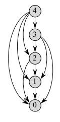
• The subproblem graph encapsulate set of subproblems that need to be solve in order to solve the current problem.
• The `n=4` graph for rod-cutting is drawn above.
• The graph contains an edge from `x` to `y` if determining an optimal solution for subproblem `x` involves directly considering an optimal solution for subproblem `y`.
• It is like a reduced version of the recursion tree for the top-down recursive method.
• The bottom-up method consider the vertices of the subproblem graph in such an order that we solve the subproblems `y` adjacent to `x` before we solve `x`.
• The size of the above graph can often be used to determine the run time of the dynamic programming problem. The run-time is typically the sum of the times to solve each of the subproblems once.

Reconstructing a solution

• Our DP solutions to rod-cutting return the value of an optimal solution, but they do not return an actual solution: a list of piece sizes.
• We can extend the dynamic-programming approach to record not only the optimal value, but also a choice that led to that value.
• Using this, we can readily print an optimal solution.

PRINT-CUT-ROD-SOLUTION

PRINT-CUT-ROD-SOLUTION(p,n)
1 (r,s) = EXTENDED-BOTTOM-UP-CUT-ROD(p,n)
2 while n > 0
3    print s[n]
4    n = n - s[n]

EXTENDED-BOTTOM-UP-CUT-ROD(p, n)
01 let r[0..n] and s[0..n] be new arrays
02 r[0] = 0
03 for j = 1 to n
04    q = -infty
05    for i = 1 to j
06       if q < p[i] + r[j - i]
07            q = p[i] + r[j - i]
08            s[j] = i // record the best 1st split for each subproblem 
09    r[j] = q
10 return r and s

Longest Common Subsequence

• Biological applications often need to compare DNA of two (or more) different organisms.
• A strand of DNA consists of a sequence of bases which can be one of four different types which we will call A, C, G, T.
• The DNA of one organism may contain the sequence:
  `S_1` = ACCGGTCGAGTGCGCGGAAGCCGGCCGAA, and of another may contain
  `S_2` = GTCGTTCGGAATGCCGTTGCTCTGTAAA.
• We may want to compare strands to say determine how similar the two organisms are.
• One could check if one string was a substring of the other.
• Alternatively, we could say two strands are similar if the number of changes needed to map one sequence to the other was small.
• Yet another way to measure similarity is by finding a third strand `S_3` in which the bases in `S_3` appear in each of `S_1` and `S_2`. We require the bases to appear in the same order but not necessarily adjacent to each other.
• The longer the strand `S_3` we can find, the more similar `S_1` and `S_2` are. In our example, the longest strand `S_3` is GTCGTCGGAAGCCGGCCGAA
• We call this the longest common subsequence.

Formalizing the LCS

• Given a sequence `X = langle x_1, x_2, ..., x_m rangle`, a sequence `Z = langle z_1, ... z_k rangle` is a subsequence of `X` is there is a strictly increasing sequence `langle i_1, .. i_k rangle` of indices of `X` such that for all `j = 1,2, ..., k`. `x_(i_j) = z_j`.
• For example, `Z = langle B, C, D, B rangle` is a subsequence of `X = langle A,B, C, B, D, A, B rangle` with corresponding index sequence `langle 2, 3, 5, 7 rangle`.
• Given two sequences `X` and `Y`, we say that a sequence `Z` is a common subsequence of `X` and `Y` if `Z` is a subsequence of both `X` and `Y`.
• For example, `langle B, C, A rangle ` is a common subsequence to `X = langle A,B, C, B, D, A, B rangle` and `Y = langle B, D, C, A, B, A rangle`.
• It is not a longest common subsequence since `langle B, C, B, A rangle` and `langle B, D, A, B rangle` are longer (these two are in fact longest common subsequences (LCSs)).
• The longest-common-subsequence problem is
  Input: Two sequence `X = langle x_1, x_2, ..., x_m rangle` and `Y = langle y_1, .. y_n rangle`.
  Output: A maximum-length common subsequence of `X` and `Y`.
• Notice the answer may not be unique. We will show how to solve this problem using a DP approach. This time let's spell out that we are following the four step procedure for coming up with DP solutions mentioned at the beginning of lecture.

Step 1: Characterizing an LCS

• A brute force solution to the LCS problem enumerates all possible subsequences of `X` and checks each to see if it is also a subsequence of `Y`. If `X` has length `m`, there are `2^m` choices of subsets of indices `{1, ..., m}`. So this will be an exponential time algorithm.
• Let `X = langle x_1, x_2, ..., x_m rangle`, define the `i`th prefix of `X`, `X_i`, to be the sequence `langle x_1, ... x_i rangle`.
• For example, if `X = langle A,B, C, B, D, A, B rangle` then `X_4 = langle A, B, C, B rangle` and `X_0` is the empty sequence.
• The LCS problem has an optimal-substructure property given by the following theorem.
  Theorem. Let `X = langle x_1, x_2, ..., x_m rangle` and `Y = langle y_1, .. y_n rangle`, and let `Z=langle z_1, ... z_k rangle` be any LCS of `X` and `Y`. Then:
  1. If `x_m = y_n`, then `z_k = x_m = y_n` and `Z_(k-1)` is an LCS of `X_(m-1)` and `Y_(n-1)`.
  2. If `x_m ne y_n`, then `z_k ne x_m` implies that `Z` is an LCS of `X_(m-1)` and `Y`.
  3. If `x_m ne y_n`, then `z_k ne y_n` implies that `Z` is an LCS of `X` and `Y_(n-1)`.
• Notice `X_(m-1)` and `Y_(n-1)` are natural subproblems.