Outline

• RB-Delete
• Quiz
• Dynamic Programming

Introduction

• Last week, we were talking about red black trees as a variation of binary search trees that stayed balanced.
• RB-trees are BSTs where each node has a color red or black. The root and leaves are black, for any node the paths from that node to a leaf always traverse the same number of black nodes, and the children of a red node must both be black.
• Thus, each of the dynamic set operations for RB-trees would be `O(log n)`.
• We said one problem though was after and insert or delete if we used the usual BST code the resulting tree may no longer be red-black.
• We showed in the case of insert that if the node inserted is colored red, that only the root is black or the children of a red node must be black properties might be violated. We then gave a loop that would allow us to push the single violation of the rb property up to the root of the tree and there we said how to fix it.
• We start today by trying to come up with a similar fix for delete.

RB-tree Transplant

• Our starting point for red black tree deletion will be BST deletion.
• Recall, for BST deletion we needed to be able to replace a subtree of BST tree with a different subtree using an operation called TRANSPLANT.
• For RB-trees we need to modify this procedure slight so as to handle nil pointers as we do for RB-trees:

  RB-TRANSPLANT(T, u, v) //replaces subtree u of T with v
  1 if u.p == T.nil
  2    T.root = v
  3 elseif u == u.p.left
  4    u.p.left = v
  5 else u.p.right = v
  6 v.p = u.p
  

RB-DELETE

• If we used the original BST delete code and the color of the `y` node that needed to be manipulated happened to be red, then the existing code would actually still produce a red black tree.
• That is basically what the code below implements.
• If the node we need to manipulate happened to be black, then we need to run some fix-up code on the tree which we describe in a moment.
• Below is the basic procedure:

  RB-DELETE(T,z)
  01 y = z
  02 y-original-color = y.color
  03 if z.left == T.nil // first handle z has only 0 or 1 child cases
  04    x = z.right
  05    RB-Transplant(T, z, z.right)
  06 elseif z.right == T.nil
  07    x = z.left
  08    RB-TRANSPLANT(T, z, z.left)
  09 else y = TREE-MINIMUM(z.right) //both children exist case
  10    y-original-color = y.color //remember color of manipulated y
  11    x = y.right
  12    if y.p == z
  13       x.p = y
  14    else RB-TRANSPLANT(T, y, y.right)
  15       y.right = z.right
  16       y.right.p = y
  17    RB-TRANSPLANT(T, z, y)
  18    y.left = z.left
  19    y.left.p = y
  20    y.color = z.color
  21 if y-original-color == BLACK
  22     RB-DELETE-FIXUP(T,x)
  

RB-DELETE-FIXUP(T,x)

• If the node `y` of the last slide were black, three problems may arise, which our fix up code would need to remedy
  1. If `y` had been the root and a red child of `y` becomes the new root, we will have violated property 2.
  2. If both `x` and `x.p` are red, then we have violated property 4.
  3. Moving `y` within the tree causes any simple path that previously contained `y` to have one fewer black nodes, violating property 5.
• You could imagine fixing the last problem by saying that node `x` now occupies `y`'s original position but has an "extra" black property (so a node can either be double black or red and black). Our fixup procedure will push the node that needs to have this property up the tree until we get to the root and then solve the problem.
• Let's look at the procedure to fix these issues:

  RB-DELETE-FIXUP(T,x)
  01 while x != T.root and x.color == BLACK
  02    if x == x.p.left
  03        w = x.p.right
  04        if w.color == RED
  05            w.color = BLACK      //case 1
  06            x.p.color = RED      //case 1
  07            LEFT-ROTATE(T, x, p) //case 1
  08            w = x.p.right        //case 1
  09        if w.left.color == BLACK and w.right.color == BLACK
  10            w.color = RED //case 2
  11            x = x.p       //case 2
  12        else if w.right.color == BLACK
  13               w.left.color = BLACK //case 3
  14               w.color = RED        //case 3
  15               RIGHT-ROTATE(T, w)   //case 3
  16               w = x.p.right        //case 3
  17           w.color = x.p.color         //case 4
  18           x.p.color = BLACK           //case 4
  19           w.right.color = BLACK       //case 4
  20           LEFT-ROTATE(T, x.p)         //case 4
  21           x = T.root                  //case 4
  22    else (same as then clause with "right" and "left" exchanged)
  23 x.color = BLACK 
  

How Fixup code works

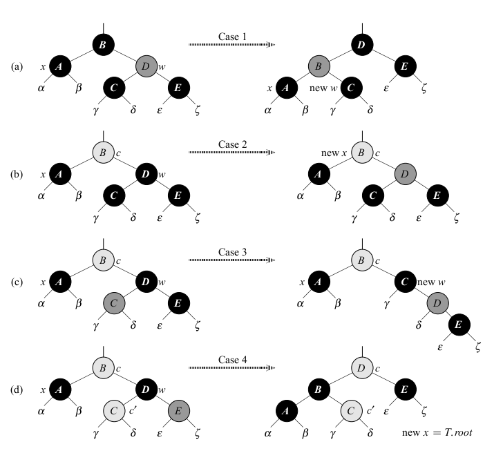
• We are only going to look at how property 5 is restored by the fix up code as we went into a lot of detail on insert last day.
• The four cases in the previously slides code are used to handle the four kinds of trees illustrated above. Darkly shaded nodes are red, light shaded are allowed to be either red or black without affecting things.
• In each case the transformation we do preserves the number of black nodes.
• Case 1 is where x's sibling `w` is red. Since `w` must have black children, we can switch the colors of `w` and `x.p` and then perform a left rotation on `x.p` without violating any red black properties. The new sibling of `x` is one of `w`'s children prior to the rotation, is now black, and thus we have converted case 1 into case 2, 3 or 4.
• Case 2, 3, 4 are four occur when `x`'s sibling `w` is black; they are distinguished by the color of `w`'s children.
• In Case 2, both children are black. In this case, we can change `w` to red, and the two subtrees will be balanced and we move the node that might have "extra" blackness up to the parent.
• Case 3 occurs when the left child of `w` is red, but the right child is black. The operation we do then changes the tree so that the right child is red, and the left child may be either red or black.
• Case 4 occurs when `x`'s sibling `w` is black and `w`'s right child is red. By making some color changes and performing a left rotation on `x.p` we remove the extra black on `x`, making it singly black, without violating any of the red black properties. Setting `x` to be the root causes the while loop to terminate.
• The runtime of fixup and delete is bounded by the height of the tree so will be `O(log n)`.

Quiz (Sec 5)

Quiz (Sec 6)

Dynamic Programming

• Dynamic Programming solves problems by combining solutions to subproblems.
• It differs from divide-in-conquer, in that in divide and conquer the sub-problems didn't overlap, where they might in the dynamic programming setting.
• So it could still be possible to use divide and conquer in the dynamic programming setting, but we may be resolving problems we have already done and be doing extra work. In contrast, dynamic programming solutions solve each subproblem only once.
• Dynamic programming is typically applied to optimization problems.
• Such problems can have many possible solutions. Each solution has a value, and we wish to find a solution with the optimal (minimum or maximum) value.

Developing a Dynamic Programming Algorithm

In developing a dynamic-programming algorithm, we typically follow a sequence of four steps:

1. Characterize the structure of an optimal solution.
2. Recursively define the value of an optimal solution.
3. Compute the value of an optimal solution, typically in a bottom-up fashion.
4. Construct an optimal solution from the computed information.

Rod Cutting

• Suppose we buy long steel rods and we want to cut them into shorter rods which we then sell.
• Suppose we charge `p_i` dollars for a rod of length `i` which is always an integer.
• The rod cutting problems is
  Input: A rod of length `n` and a table `p_i` for `i=1, ...,n`.
  Output: The maximal revenue `r_n` obtainable by cutting up the rod and selling the pieces.
• Notice if `p_n` is large enough, it might make sense not to cut the rod at all!

Example Rod Cutting

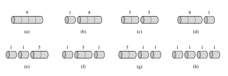
• Above we see all the ways to cut up a rod of 4inches in length.
• Here `p_1 = 1, p_2 = 5, p_3 =8`, and `p_4 = 9`.
• We see that a cut into two 2-inch pieces produces revenue `p_2 + p_2 = 5 + 5 = 10`, which is optimal.

Rod Cutting Discussion

Top-down Rod Cutting

• Using our equation from the last slide we can solve the rod-cutting problem with the following procedure:

  CUT-ROD(p,n)
  1 if n == 0
  2     return 0
  3 q = - infty
  4 for i = 1 to n
  5     q = max( q, p[i] + CUT-ROD(p, n-i ))
  6 return q
  

• This code is very inefficient. Next day we will solve it with dynamic programming!