Finish Lighting, Geometric Modeling

CS116b/CS216

Chris Pollett

Apr 16, 2014

Outline

We have been talking about lighting models suitable for high quality rendering using techniques like ray tracing.
At the end of last day we observed that our method of modeling total light based as sum over light from different numbers of bounces in the scene:
`L^t = L^e + L^1 + L^2 + L^3 + ...`
yields the equations
`= L^e + BL^t`
`L^t(tilde x, vec v) = L^e(tilde x, vec v) + int_H dw f_(tilde x, vec n)(vec w, vec v) L^t(vec w, tilde x) cos (theta)`

called the rendering equation.
We then went over some starter code for HW4.
Today, we start by describing how model effects that come when physical camera can be modeled in our lighting setup.
Then we look at techniques for solving the rendering equation before we switch to the topic of geometric modeling.

The image that a real world camera captures is `L^t` the total equilibrium light distribution of light in the scene.
For a pinhole camera, the film plate captures the incoming radiance at each pixel/sample location along a single ray through the pinhole.
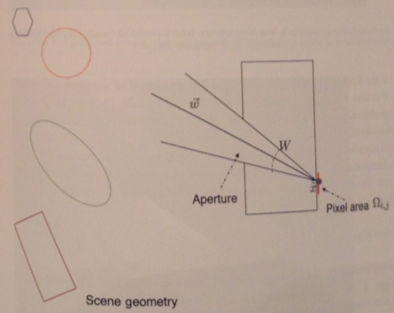
In a non-pinhole, physical camera, we have a fixed aperture and a finite shutter speed which capture a finite amount of photons on our sensor plate as illustrated in the first picture above.
We can model the pixel count received over time `T` at pixel `(i,j)` of sensor size `Omega_(i,j)` with spatial sensitivity, `F_(i,j)`, via the integral
`int_T dt int_(Omega_(i,j)) dA int_W dw F_(i,j)(vec w, tilde x)L^t(vec w, tilde x) cos (theta)`.
Here `W` is the wedge of vectors coming in from the aperture toward the film point.

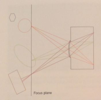
To organize light, a real-world camera has a lens placed in front of the aperture.
One model for such lenses is known as the thin lens model. The geometry of this model is illustrated by the second picture above.
The effect of the lens in this model is to keep objects at a certain depth in focus (the circle above). Objects not of this depth appear blurred.
In our equation this blurring occurs because of the integral `int_W`, the wedge into a point will actually be sampling light from several points of the surfaces it came from rather than one.
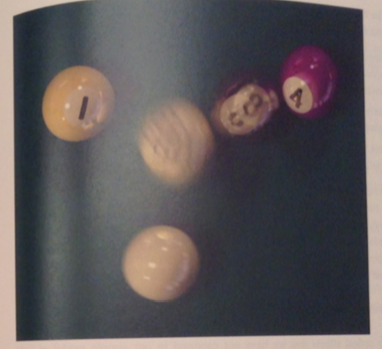
We have seen how integration over the pixel area, can be used for anti-aliasing
Integration over shutter duration can be used to simulate motion blur (see above).
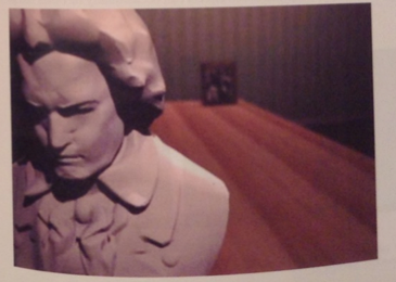
Integration over the aperture produces focus and blur effects, also called depth of field effects (last image above).

The computation of the total equilibrium light distribution is a `L^e` plus a sum over the `L^i`'s.
Each increase in `i` involves an additional nesting of the number of integrals that need to be integrated.
Rather than compute these integrals, we typically approximate them as a sum over some set of samples of the integrand.
Most of the work in photo-realistic rendering involves figuring out the best ways to approximate these integrals.
Some common approximation techniques are:
- To use randomness to choose samples, This avoids noticeable patterns in the errors during approximation.
- Reuse computations -- if we know the irradiance pattern at a point, we might be able to share this data to simplify the computation of irradiance at nearby points.
- Use cut-offs, so that we don't follow rays that don't carry much radiance.

Out simple model of light and reflection does not capture all possible optical effects.
For example, atmospheric volumetric scattering which occurs when light passes through fog, is not capture by our model.
Also, fluorescence, which occurs when surfaces absorb light and this re-emit this energy (often at a different wavelength), is also not covered by our model.
Our model also doesn't cover polarization and diffraction effects, although we did talk about anisotropic materials last semester in a different setting.
Finally, our model also doesn't handle subsurface scattering. This happens when light enters at a point, bounces around inside the surface, and comes out over a finite region around the point of entrance. This kind of scattering has the effect of softening the surface as might be observed in pictures of skin or marble.

In computer graphics we need ways to represent shapes as data structures which could be coded.
Geometric modeling is the topic of how to come up with such data structures that also us to represent, create, and modify shapes.
Our next topic today is a basic introduction to common approaches used in geometric modeling.

The easiest to describe representation is to represent an object as a triangle soup: a set of triangles each described by three vertices.
We can then reorganize this data to reduce redundancy.
For example, we might store each vertex only once, even when it is shared by many triangles, and use an index buffer.
We might use triangle strips or triangle fans to specify the triangles and their connectivity more compactly.
Related to triangle soups one can also have quad soups and polygon soups.
At hardware rendering time, these polygons are typically diced into triangles and drawn using a usual triangle rendering pipeline.
Triangle geometry can be created in a number of ways, and many geometric modeling tools can be used to output triangles.
We will describe later some techniques for tessellating a surface into triangles.

One thing lacking in triangle soups is a way to "walk along" the geometry
One cannot usually in constant time figure out which triangles meet at an edge or which triangles surround a vertex.
Walking along a mesh can be useful, for example, if we want to make the geometry smoother or if one wants to model a physical process over the geometry.
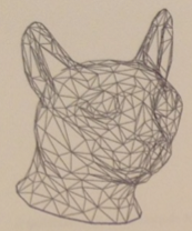
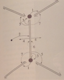
A mesh is data structure representation that organizes the vertex, edge, and face data so that these queries can be done quickly.
Above we can see an example of what might be stored in a mesh (winged-edge representation).