On Monday, we went over the shader code for cube maps. I have now added to the last lecture code
in OpenGL land for loading in the images to be used in the cube map and updated the project file accordingly.
We then talked about projection texture mapping and started talking about multipass texture mapping.
Our first example of this was dynamic reflection mapping: we first render the scene as seen from say the center of the mirrored object
in the six canonical directions of a cube, making a cube map from these images.
Then we use this cube map when we draw the reflective surface in a second pass.
We start today by looking at another multi-pass technique called shadow mapping.
Shadow Mapping
When we modeled materials last semester, the color at a point did not depend on the rest of the geometry of the scene.
In the real world, there could be an object between the light source and the point we are trying to figure out the color of.
I.e., the point we are calculating is in the shadow of the blocking object.
To simulate this effect we can use a multipass technique called shadow mapping.
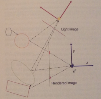
We first create and store a z-buffered image from the point of view of the light source.
We then compare this with what we see in the eye view. If a point observed by the eye is not observed by the light, it must be occluded,
and we should draw the point in the shadow.
Shadow Mapping Details
In the first pass, we render into a frame buffer object (FBO) the scene observed from some camera whose origin coincides with the position of the point light source. This camera transform would be:
`[[x_tw_t],[y_tw_t],[z_tw_t],[w_t]] = P_sM_s[[x_O],[y_O],[z_O],[1]]`
Where `P_s` and `M_s` are the projection and modelview matrices for this vantage.
In the FBO, we store not the color of the point but rather its `z_`t value.
Because of z-buffering, the data stored at a pixel will represent the `z_t` value of the geometry closest point to the light source.
The FBO is then transferred to a texture
During the second rendering pass, we render the image from the eye's viewpoint, but for each pixel, we check to see if the point we are observing was observed by the light or if it was blocked.
To do this, we use the same calculation we used for projector texture mapping.
In the fragment shader, we can obtain `x_t`, `y_t`, and `z_t` associated with the point `[[x_O],[y_O],[z_O],[1]]` of the point on our object.
We can then compare these values with the `z_t` stored in the texture. If the values agree to within some tolerance, then it wasn't occluded, otherwise, we treat the point as being in the shade.
Modeling
Before we start talking about SDL, we are going to have a brief interlude where we begin one of the themes of this semester: modeling of objects and scenes.
To start we are going to talk about the simplest kinds of objects and how to represent them: polyhedra and quadrics.
Polyhedra
A polyhedron (singular of polyhedra) is a 3D solid object with flat faces whose boundaries are given by straight edges.
We will often be interested in the case where the faces are convex polygons.
Here convex means that whenever I have two points within a
face, the points along edge between them also are in the face.
A polygon is the figure enclosed by a a finite chain of edges whose first edge's, first vertex, and whose last edge's last vertex are the same.
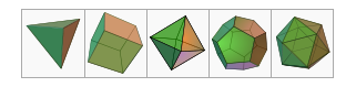
Some examples of convex polyhedra are: tetrahedron, pyramid, cube, octohedron, dodecahedron, and icosahedron.
Representing Convex Polyhedra
Convex polyhedra can be represented as a sequence of triangles.
To see this it suffices to represent the polygons of each face with a triangle.
But for a convex polygon, this is easy: Just add edges from the first point in the list to each other point in the list and this, together with the edges of the original polygon, will give a triangulation.
Given the coordinates of the vertices in a convex polyhedra, we could use this technique to make index buffer objects for theses triangles.
Alternatively, we could use a natural triangle fan representation and have a sequence of these one for each face.
OpenGL supports drawing triangle fans and more complicated shapes then the GL_TRIANGLES we have used so far.
The syntax looks like:
glBegin(GL_TRIANGLE_FAN);
// a sequence of glVertex* (here * is the type like f for float) calls
glEnd();
Other possibilities are: GL_TRIANGLES,
GL_TRIANGLE_STRIP, GL_TRIANGLE_FAN,
GL_QUADS, etc.
It should be noted if we weren't using shaders, we could make use of the old-style GLUT calls for a number of built-in objects: glutWireTetrahedron(); , glutSolidTetrahedron(); glutWireCube(); etc.
Curved Surfaces
One step up in complication from polyhedra are curved surfaces represented by a quadratic equation. I.e., quadrics.
The simplest of these are:
Sphere
which is given by the equation: `x^2 + y^2 + z^2 = r^2` where `r` is the radius. Let `theta in (-pi,pi]` be a rotation about the `y` axis, and let `phi in (-pi/2,pi/2]` be a rotation of the result about the `z`-axis. In polar coordinates:
`x = r cos phi sin theta`, `y = r sin phi sin theta`, and `z= r cos theta`.
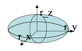
Ellipsoid
which are given by the equation: `(x/r_x)^2 + (y/r_y)^2 + (z/r_z)^2 = 1` where `r_x`, `r_y`, `r_z` represent how much the basic
sphere shade has been stretched with respect to each axis. In polar coordinates, `x = r_x cos phi sin theta`, `y = r_y sin phi sin theta`, and `z= r_z cos theta`.
Torus
The solid of revolution given by rotating a circle around the origin at some radial distance `r_(text(axial))`. In polar coordinates: `x=(r_(text(axial)) + r cdot cos phi) cdot cos theta`, `y=(r_(text(axial)) + r cdot cos phi) cdot sin theta`, and `z = r cdot sin theta`.
Quadrics can be generalized to something known as a super-quadric which generally flatten or concavifies the curve around the exterior of the quadric. For example, a super-wllipsoid is given by the equation: `(x/r_x)^(2/s_1) + (y/r_y)^(2/s_2) + (z/r_z)^(2/s_1) = 1`
Representing Quadrics
GLUT has built-in functions for quadrics such as glutWireSphere(r, nLongitude, nLatitude); and glutSolidSphere(r, nLongitude, nLatitude)
You will also notice the geometry_maker.h header has code for converting a sphere to a set of triangles.
The GLUT functions give us a hint at how this is done. We imagine the surface is a split into a sequence of cylinders. Each cylinder can be split into a sequence of rectangles and hence triangles. In the case of the sphere and ellipsoid we also have a triangle fan for the top and bottom.
Fractals
A fractal is a mathematical set which displays a self-similar pattern.
We will use fractals in computer graphics to make models things in a "natural way".
That is, we will use fractals to make models for things like branches in trees, leaves, terrain, etc.
Initiator and Generator
A simple fractal can be made using two components: an initiator and a generator.
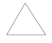
The initiator is a starting shape `S_0`:
Starting from shape `S_n`, to make shape `S_(n+1)`, we apply a generator to each subcomponent of `S_n`. In this case,
our subcomponents are edges.
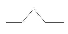
Here is our generator:
Applying our generator to each edge of `S_0` yields:
If we kept going, in this case, we would get something that looks like a snowflake.
After iterator some desired number of steps we stop. We might also apply a final shape for the last step. For example,
we can use this idea to generate stems of flowers and then for the last iteration replace some of the final stems with flowers.
More on Self Similar Fractals
It is legal to use generators which are not connected:
Applying the above generator to the interval `[0,1]` gives Cantor's dust:
an example of a measure 0, uncountable set.
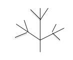
Simple plants and trees can be modeled with fractal techniques.