Introduction

On Monday, we started talking about a lighting model suitable for use in ray-tracing.
We defined the radiant flux, `Phi(W, X)`, of a wedge `W` through a sensor `X` and said that it was measured in watts.
We then defined irradiance, `E_(vec n)(W, tilde x)`, as the limiting case as we let planar sensor with normal `vec n` shrink in size to the point `tilde x`.
Similarly, if we also shrink the wedge angle down to a single vector `vec w`, we get a quantity called outgoing radiance:
`L(vec w, tilde x) := L_(- vec w)(vec w, tilde x) = (L_(vec n)(vec w, tilde x))/(cos theta)`
where `theta` is the angle between `vec n` and `- vec w`.
We can going backward and forwards from outgoing radiance to radiant flux and vice-versa via the equations:
`Phi(W, X) = int_X dA int_W dw L(vec w, tilde x) cos(theta)`
where `dw` is a differential measure of steradians, and
`L(vec w, tilde x) := 1/(cos theta) lim_(W rightarrow vec w) 1/(|W|)(lim_(X rightarrow tilde x) (Phi(X, W))/(|X|))`
Finally, we said that `L(vec w, tilde x) = L(vec w, tilde x + vec w)`. The book has a proof but we will skip it.
Now that we have the basic quantities that we measure when handling light, we can see what happens to light under reflections, and other lighting phenomena -- all of which we can use when writing a ray-tracer.

Reflection

Suppose light comes in from some wedge `W` centered about a direction `vec w` and that it is then reflected.
To keep things simple, we assume that all reflection is pointwise.
We want to measure the light that is reflected out along `V`, some wedge of outgoing directions around an outgoing vector `vec v`.
We will describe the bouncing behavior of this light as some function `f` which is a ratio of incoming to outgoing light.
Two properties we want for this ratio are:
1. It converges as we use smaller and smaller incoming and outgoing wedges
2. And the ratio (for small enough wedges) does not depend on the size of the wedges.
Let's look at a distribution function which solve this.

Most materials other than pure mirrors or lenses have a diffusing behavior: For any fixed incoming light pattern, the outgoing light measured along any outgoing wedge changes continuously as we rotate the wedge.
So if the outgoing wedge `V` is doubled in size, we see roughly twice the outgoing flux.
If we want the numerator of our ratio `f` not to depend on the size of `V`, this suggest the numerator should be measure in units of radiance. Let this outgoing measurement be denoted `L^1(tilde x, vec v)`.
Similarly, for most materials (excluding perfect mirrors and lenses), for any fixed in coming light pattern, the outgoing light measured along any outgoing wedge varies continuously as we rotate this wedge.
So if we double the size of the incoming `W` and hold the outgoing `V` fixed, the amount of outgoing flux will roughly double.
To get a ratio that does not depend on the size of `W`, this suggest using incoming light units of irradiance.
The above discussion suggests measuring `f` as
`f_(tilde x, vec n)(W, vec v) = (L^1(tilde x, vec v))/(E_(vec n)^e(W, tilde x))`
`= (L^1(tilde x, vec v))/(L_(vec n)^e(W, tilde x)|W|)`.
Here `L^e` refers to photons that have been emitted by some light source and have not yet bounced.
This `f` is called the bidirectional reflection distribution function or BRDF.

The simplest BRDF is the constant function `f_(tilde x, vec n)(W, vec v) =1`.
This represents the behavior of a diffuse material. The outgoing radiance at a point does not depend on `vec v` the outgoing direction at all.
More complicated BRDFs can be derived from a variety of methods.
- We can hack up some functions that makes our materials look nice in picture. This is what we did last semester when we were talking about materials.
- We can derive the BRDF using various physical assumptions and statistical analysis. This involves a deeper understanding of the physics of light and materials.
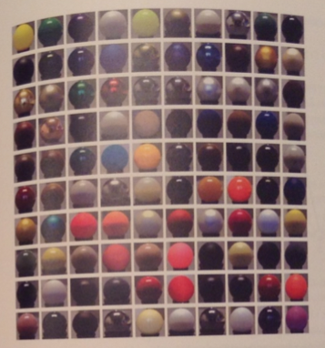
- We can build devices that actually measure the BRDF of real materials. This can then be stored in a big table or approximated using some functional form. The above picture was made by placing various materials in such a capturing device.

Suppose we want to compute outgoing `L^1(tilde x, vec v)` at a point on a surface with normal `vec n` due to light coming in from the hemisphere, `H`, above `tilde x`. This light may later fall on an object which we want to calculate during ray-tracing.
Suppose further `H` is broken into a set of finite wedges `W_i`. Then we can compute the reflected light using the sum
`L^1(tilde x, vec v) = sum_i|W_i|f_(tilde x, vec n)(W_i, vec v) cdot L_(vec n)^e(W_i, tilde x)`.
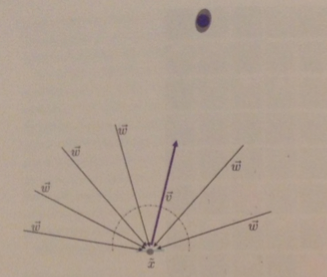
In the limit as the wedges get smaller we get the reflection equation:
`L^1(tilde x, vec v) = int_H dw f_(tilde x, vec n)(vec w, vec v) L^e(vec w, tilde x) cos (theta)`.
This diagram above show this equations in action: the outgoing radiance is computed as an integral of all the incoming rays.

Pure mirror reflection and refraction are not easily modeled using BRDF.
In a mirrored surface, `L^1(tilde x, vec v)`, the bounced radiance along a ray, depends only on `L^e(-B(vec v), tilde x)`, the incoming radiance along a single ray. Here `B` is the bounce operator we had earlier.
Doubling the size of an incoming wedge that includes `-B(vec v)` has no effect on `L^1(tilde x, vec v)`.
For mirror materials, this reflection behavior can be modeled as
`k_(tilde x, vec n)(vec v) = (L^1(tilde x, vec v))/(L^e(-B(vec v), tilde x))`
where `k_(tilde x, vec n)(vec v)` is some material coefficient.
So in this case we replace our reflection equation with
`L^1(tilde x, vec v) = k_(tilde x, vec n)(vec v) cdot L^e(-B(vec v), tilde x)`.
This is actually easier to calculate in that it doesn't involve an integral.
Refraction happens when light passes between different mediums each with its own index of refraction. For example, light going into air coming out of glass.
The rays bend in this case according to geometric rules:
`(sin theta_1)/(sin theta_2) = v_2/ v_1 = n_2/n_1`
here `theta_1` is the angle of incidence and `theta_2` is the angle of refraction, `v_i`'s are the speed of light in the two different media, and `n_i`'s represent indices of refraction.
As with reflection the radiance along each outgoing ray is affected by the radiance of a single incoming light ray.

The reflection equation can be used in a nested fashion to describe how light bounces around an environment multiple times.
Such descriptions typically result in definite integrals that need to be calculated.
In practice this computation is done by some sort of discrete sampling over the integration domain.
We next start to look a this is more detail.
We use `L` with no arguments to represent the entire distribution of radiance measurements in a scene due to a certain set of photons.
We use `L^e` to represent unbounced photons (emitted) and `L^i` to represent the radiance of photons which have bounced exactly `i` times.

In OpenGL, our light comes not from area lights but from points lights.
Such point lights do not conform to our continuity assumptions and are not so easily represented with our units.
For point light, we simply replace the reflection equation with
`L^1(tilde x, vec v) =f_(tilde x, vec n)(-vec l,vec v)E_(vec n)^e(H, tilde x)`.